Sage Journals: Discover world-class research

Abstract

In this paper, we propose a new algorithm of mapping dynamic indoor environments. Instead of accurate but expensive laser, we employ sonar and camera to map dynamic structured indoor environments. Based on fuzzy-tuned grid-based map (FTGBM), we use two methods: sonar temporal difference (STD) and statistical background subtraction (SBS), to detect and track moving objects when mapping dynamic environments. The former is a consistency-based method realized by monitoring a sequence of temporal lattice maps for a certain number of measurement periods to detect moving objects by using sonars; and the latter is a background subtraction technique which adopts an expectation maximization (EM) learned 3-class mixture of Gaussians to model the nonstationary background relied on sufficient update during mapping process. After finding the moving objects, we propose a fuzzy-tuned integration (FTI) method to incorporate the results of motion detection into the mapping process. The simulation and experiment demonstrate the capabilities of our approach.

Keywords

Mapping tracking mobile robots

1. Introduction

Robotic mapping is referred to the process of generating spatial models of physical environments from sensor measurements through navigating in the environment. This procedure is generally regarded as one of the most important problems in the pursuit of building truly autonomous mobile robots. Over the past two decades, the field has been received considerable attention, because generation and maintenance of environmental maps are often inherently necessary for mobile robots in order to perform complex tasks in partially known or unknown environments. At present, this field has matured to a point where detailed maps of large-scale complex environments can be built in real-time, specifically indoors (Thrun, S. et al 1998a; 1998b; 2001a; 2002; Bosse, M. et al 2004). Many existing techniques are robust to noise and can cope with variety of structured environments. However, the majority of existing mapping approaches are designed for static environments. They assume that the mobile robot is the only moving object in the map world. Nevertheless, the real worlds, where robots are deployed, are usually dynamic. That is, some objects in the environments do often change states over time. In an office, for instance, the location of desks may have been changed, and doors may be opened or closed, etc. In particular, to map a crowded environment, there also exits multiple moving objects in the perceptual range of the robot. For example, there may be many people walking through a corridor of an office building during office hours who are within the sensor range of the robot during the mapping process. In this context, such people moving in or out the scene will have a serious influence on the resulting map since it would contain evidence about these people at the corresponding locations. But when the robot later returns to this location and scans the area a second time using such localization methods as (Thrun, S. et al 2001b; Fox, D. et al 1999), the pose estimates would be less accurate, because the new measurements do not contain any features corresponding to those people, thus resulting in spurious objects in the map and consequently affects the future tasks (Hähnel, D. et al 2003a; 2003b). Therefore, an autonomous mobile robot should be equipped with the capacity to be conscious of the changes around it and to filter out the spurious models of moving objects when building maps and to constantly update its map of the environment, if it is going to perform services in real world.

In this paper, we extend our pervious work (Ip, Y.L. et al 2002; Chow, K.M. et al 2002) which is able to model the static environments and propose a mapping technique allowing a mobile robot to map the dynamic environments, with the assumption that the odometry is perfect, so that localizatoion problem is not considered in this work. Particularly, we use fuzzy-tuned grid-based map (FTGBM) (similar idea as in our previous work (Chow, K.M. et al 2002)) to model the environment. We suggest two methods: sonar temporal difference (STD) and statistical background subtraction (SBS) to detect moving objects. The former is a consistency-based method realized by monitoring a sequence of temporal lattice maps for a certain number of measurement periods to detect moving objects by using sonars; and the latter is a statistical background subtraction technique which adopts an expectation maximization (EM) learned 3-class mixture of Gaussians to model the nonstationary background based on sufficient update during mapping process. After obtaining the motion information, we propose fuzzy-tuned integration (FTI) to incorporate the results of above two types of motion detection to filter the moving objects out of the resulting map. Additionally, since Bayesian update rule is used in FTGBM, our approach also has the capability to estimate and update the states of the dynamic objects in robot workplace.

The rest of this paper is organized as follows. After discussing the related work in the following section, we will briefly present basic notation and definition about the fuzzy system and fuzzy-tuned grid-based map building method in Section 3. We will describe the sonar temporal difference by sonar sensor in Section 4 and statistical background subtraction by camera in Section 5, and then report the fuzzy-tuned integration to incorporate the motion tracking results into the resulting map in Section 6. And Section 7 will contain our simulation and experiments to illustrate the capabilities and the robustness of our approach. Finally, conclusions and future work will be presented in Section 8.

2. Related Work

Approaches to mapping problem can be roughly classified into two major paradigms: occupancy grid-based maps and topological maps. The occupancy grid-based maps, like our previous work (Chow, K.M. et al 2002) are generated from stochastic estimates of the occupancy state of an object in a given cell. It is rather easy to construct and maintain them, whereas topological maps are graph-like spatial representations (Remolina, E. & Kuipers, B. 2004). Nodes in such graphs correspond to distinct situations, places, or landmarks (such as corners). They are connected by arcs if there has a direct path between them. Furthermore, Thrun, S. (1998a) successfully integrated these two paradigms to build a metric-topological map, thus gaining the advantages from both methods. However, all these approaches assume that the environment is almost static during the mapping process, although they can tackle a certain mount of noise in the sensor data. But in dynamic environments where moving objects are appearing or disappearing in the perceptual range and states of the objects are changing over time, robots have to be equipped additional ability to deal with such additional noise comparing with the static environments. Otherwise, the resulting maps can not be usable for localization or navigation.

Recently, there has been work on updating maps in dynamic environments. Thrun, S. et al. (2000) and Burgard, W. et al. (1999) update a given static map using the most recent sensor information to deal with people in the environment. Fox D. et al. (1999) propose a filtering technique to identify range measurements that do not correspond to the given world model, and then to update the robot position using only those measurements which are with high probability produced by known objects contained in the map. Montemerlo et al. (2002) present an approach to simultaneous localization and people tracking. More recently, there also exist several approaches to mapping in dynamic environments which contain moving objects in perceptual range of the robots. Biswas, R. et al. (2002) and Anguelov, D. et al. (2002) derive an approximate Expectation-Maximization (EM) algorithm for learning object shape parameters at both levels of the hierarchy, using local occupancy grid maps for representing shape. Andrade-cetto et al. (2002) combine the landmark strength validation and Kalman filtering for map updating and robot position estimation to learn moderately in dynamic indoor environments. Montemerlo et al. (2002a) employ a Rao-Blackwellized particle filter to solve the simultaneous localization and people tracking problem based on a prior accurate map of the corresponding static environment, which is similar with FastSLAM (Montemerlo et al. (2002b)). Hähnel et al. (2003) present a probabilistic approach to map populated environments by using Sample-based Joint Probability Data Association Filters (SJPDAFs) to track people in the data obtained with the laser range scanners of the robot like Schulz, D. et al. (2001; 2003). The results of the people tracking are integrated into a scan alignment process and into the map generation process, thus filtering out the spurious objects in the resulting maps. Wang C.-C. (2004) solves the problem of simultaneous localization, mapping and moving object tracking in crowded urban environments. He establishes a mathematical framework to integrate SLAM and DATMO (Detection and Tracking Moving Objects). The idea is to identify and keep track of moving objects in order to improve the quality of the map. Wolf et al. (2005) propose an online algorithm for SLAM in dynamic environments, which is based on maintaining two occupancy grid maps: one for static objects and another for dynamic ones, and a third landmark map with which localization is solved. This method is limited to moderately dynamic indoor environments, especially the narrow assumption of localization implementation. But the algorithm has advantages that it is robust to detect dynamic entities both when they move in and out robot's field of view.

However, virtually all state-of-art approaches use SICK scanning laser range-finders. While the SICK is ideal for this because of the accurate and detailed range information provided, there are drawbacks. In particular, the SICK laser sanner is expensive and quite heavy and bulky. It seems that these methods can not be assigned to cost effective sensor systems such as sonars.

In our work, we propose a new technique of mapping dynamic environments. We respectively use sonar sensors and camera to detect moving objects, and then fuzzy-tuned integrate the results of motion detection to filter out the moving objects from the resulting map. Additionally, we use Bayesian update rule in fuzzy-tuned grid-based map to estimate and refine the states of some dynamic objects which change slowly.

3. Fuzzy System and Fuzzy-Tuned Grid-Based Map (FTGBM)

3.1. Notation and Definition of Fuzzy System

Consider a fuzzy model with n inputs and a single output. The fuzzy rule base can be formulated as:

$R^{j_{1} j_{2} \dots j_{n}}$ : If x₁ is $A_{1}^{j_{1}}$ and x₂ is $A_{2}^{j_{2}}$ and … and xⁿ is $A_{2}^{j_{n}}$ then $y^{j_{1} j_{2} \dots j_{n}}$ is $B^{j_{1} j_{2} \dots j_{n}}$ .

x_i: The ith input variable.

$y^{j_{1} j_{2} \dots j_{n}}$ : The output variable corresponding to the rule $R^{j_{1} j_{2} \dots j_{n}}$ .

N_i: The number of fuzzy subsets of input i.

n: The number of input variables.

$A_{i}^{j_{i}}$ : The j_ith fuzzy set of input i where j_i =1, 2, …, N_i, i=1, 2, …,n.

$B^{j_{1} j_{2} \dots j_{n}}$ : The output fuzzy set corresponding to rules $R^{j_{1} j_{2} \dots j_{n}}$ where j_i=1, 2, …, N_i, i =1, 2, …, n.

${\binom{-}{o}}^{j_{1} j_{2} \dots j_{n}}$ : The center of output fuzzy set $B^{j_{1} j_{2} \dots j_{n}}$ .

$μ_{A_{i}^{j_{i}}} (x_{i})$ : The fuzzy membership function for the j_i th fuzzy set of input i.

Assuming singleton fuzzifier, product inference engine and centre average defuzzifier (Wang, T. X. 1997), and the crisp fuzzy model output ŷ is obtained as:

\hat{y} = \frac{\sum_{j_{1} = 1}^{N_{1}} \sum_{j_{2} = 1}^{N_{2}} \dots \sum_{j_{n} = 1}^{N_{n}} {\bar{o}}^{j_{1} j_{2} \dots j_{n}} \prod_{i = 1}^{n} μ_{A_{i}^{j_{i}}} (x_{i})}{\sum_{j_{1} = 1}^{N_{1}} \sum_{j_{2} = 1}^{N_{2}} \dots \sum_{j_{n} = 1}^{N_{n}} \prod_{i = 1}^{n} μ_{A_{i}^{j_{i}}} (x_{i})}

(1)

3.2. Fuzzy-Tuned Grid-Based Map (FTGBM)

We adopt fuzzy-tuned grid-based mapping technique to generate a basic global map and will update this basic map in following sections by filtering out the spurious objects and refining the dynamic object states. Here, the fuzzy-tuned grid-based map algorithm is similar with our previous work (Chow, K. M. et al 2002). Therefore, we only briefly review this algorithm to make this paper readable on its own. Interested readers may refer to (Chow, K. M. et al 2002) for further details.

In this approach, the probability distribution function (pdf) of the sonar sensor model is tuned by a set of fuzzy rules based on the maximum probability of the grid cell within the sensor cone. Similar to traditional approaches, the occupancy grid probabilities of the state s(C_i) of grid cell C_i for the environmental map P[s(C_i) = occ | x] = 0.5 means unknown or unexplored region. P[s(C_i) = occ | x] = 1 means that the grid cell G is occupied and vice-versa. The fuzzy-tuned sonar sensor model (pdf) is shown in Eq. 2, considering the example of a range sensor characterized by Gaussian uncertainty in both radial and angular directions. In Eq. 2, where

r: The sensor range measurement of the sonar sensor.

z: The true parameter space range value.

θ: The azimuth angle measured with respect to the beam central axis.

k_o: The parameter that corresponds to the space is occupied.

$σ_{r}^{2}$ : The variance of the measure.

$\bar{θ}$ : The parameter that will be tuned by fuzzy model and corresponds to the mean azimuth angle measured with respect to the beam central axis.

${σ_{θ}}^{2}$ : The parameter that will be tuned by fuzzy model and corresponds to the variance of the angular probability.

k_ε: The parameter that corresponds to the empty space and will be tuned by the fuzzy model.

{\begin{cases} i f 0 \leq x < a a n d (1 - k_{ε}) \exp (\frac{- (θ - \bar{θ})^{2}}{{σ_{θ}}^{2}}) > 0.5, \\ p (r | z, \bar{θ}) = 1 - (1 - k_{ε}) \exp (\frac{- (θ - \bar{θ})^{2}}{{σ_{θ}}^{2}}); \\ i f a \leq x < b a n d (1 - k_{o} \exp) (\frac{- (r - z)^{2}}{{σ_{θ}}^{2}})) \exp (\frac{- (θ - \bar{θ})^{2}}{{σ_{θ}}^{2}}) > 0.5, \\ p (r | z, \bar{θ}) = 1 - (1 - k_{o} \exp (\frac{- (r - z)^{2}}{{σ_{θ}}^{2}})) \exp (\frac{- (θ - \bar{θ})^{2}}{{σ_{θ}}^{2}}); \\ i f b \leq x < c a n d k_{o} \exp (\frac{- (r - z)^{2}}{{σ_{θ}}^{2}}) \exp (\frac{- (θ - \bar{θ})^{2}}{{σ_{θ}}^{2}}) > 0.5, \\ p (r | z, \bar{θ}) = k_{o} \exp (\frac{- (r - z)^{2}}{{σ_{θ}}^{2}}) \exp (\frac{- (θ - \bar{θ})^{2}}{{σ_{θ}}^{2}}) \\ o t h e r w i s e, \\ p (r | z, \bar{θ}) = 0.5 \end{cases}

(2)

A plot of $p (r ∣ z, \bar{θ})$ corresponding to sensor measurement at 0.7m is shown in Fig. 1 which fairly accurately represents the radial and angular uncertainty.

Fig. 1.

Occupancy probability $p (r ∣ z, \bar{θ})$ in 2D case

After obtaining the sonar sensor model pdf, we use Bayesian update rule (Eq. 3) to update the occupancy probabilities of the grid cells.

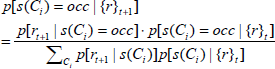
\begin{aligned} p [s (X_{i}) = o c c ∣ {r}_{t + 1}] \\ = \frac{p [r_{t + 1} ∣ s (C_{i}) = o c c] . p [s (C_{i}) = o c c ∣ {r}_{t}]}{\sum_{C_{i}} p [r_{t + 1} ∣ s (C_{i})] p [s (C_{i}) ∣ {r}_{t}]} \end{aligned}

(3)

where P[s(C_i = occ | {r}_t] is the prior occupancy grid probability of grid cell C_i based on observations {r} = {r₁, r₂, …, r_t}, P[s(C_i) = occ | {r}_t+1] is the new occupancy grid probability of grid cell C_i based on observation up to r_t+1. The fuzzy-tuned grid-based map-building algorithm is an incremental method, as most traditional mapping algorithms, i.e. it only add specific features in the map model and never removes the old features. Hence, the global map contains all the sensor information, surely including spurious models of moving objects. In order to filter out such spurious models, we use following motion detecting methods and fuzzy-tuned integrating technique, thus getting the resulting map only contains stable stationary objects.

4. Sonar Temporal Difference (STD)

The fundamental idea to identify temporal changes in the surrounding environment of a robot is to monitor a temporal sequence of spatial observations and then to determine how these observations differ from each other. An inconsistency between two temporally subsequent observations is a strong indication of a potential motion in the environment. Such inconsistency is mainly caused by dynamic objects in a dynamic indoor environment. In computer vision literature, temporal difference is simple and popular method for detecting moving objects with a static observer. However, for a moving mobile robot, it in itself is not sufficient to unequivocally identify moving objects. Here, we propose a new scheme to detect moving objects using sonar sensors called sonar temporal difference (STD) borrowing from the etymology in the computer vision literature, which is realized by monitoring sensor-based information called time-variant map (TVM) along the time axis with a certain time duration of τ (τ = nt, t is sampling time) and simultaneously filtering out the same information, i.e. stationary objects, thus obtaining the trajectories and outliers of moving objects during time span τ. Note that all the sensor information has been transformed into the same global coordinate frame.

4.1. Time-Variant Map (TVM)

Sonar temporal difference is realized by monitoring a temporal sequence of time-variant maps (TVMs). This procedure is not new and we have borrowed it from (Han, Y. et al 2001; Prassler, E. & Scholz, J. 2000). We also adopt occupancy grid model to represent time-variant map because it is easy to incorporate the result of sonar temporal difference into the resulting fuzzy-tuned grid-based map. Elfes, A. (1989) introduced the occupancy grid map. It includes the projection of the range scans on a 2D rectangular lattice and the annotation of each cell with the time tags of the measurements that fall into it. Each grid corresponds to a small spatial region in the real world.

In occupancy grid-based mapping procedure, every time that new measurements are available, a significant amount of time is spent in updating the posterior including free space or stationary object state from Bayesian update rule (Eq. 3). However, it is less important in the context of short-term motion detection since all the sensor data information is synchronically registered in fuzzy-tuned grid-based map. Hence, we only update the occupancy probabilities of those cells in local sensor cone at time t while all other cells remain untouched. Fig. 2 clearly shows the relevant transformation. It should be noted that our experimental platform is Pioneer 1 mobile robot (Active media 1998a) that only has seven sonar sensors, five in front and two at each side, separated by 15-degrees. Here, we are only concerned with the front 75-degree region. Therefore, there is only a 75-degree cone shown in Fig. 2b. We call this representation a time-variant map. Building such maps is rather simple: in each sensor measurement at time t, the cell that corresponds to the object detection is labeled with this time tag t. The tag means that the cell occupied at time t. No other cells are updated during this operation. Therefore, the temporal changing features of the environment are captured by the sequence of time-variant maps: TVM_t, TVM_t-1, …, TVM_t-n. An example of such a sequence is shown in Fig. 3(a)–(c). Note that the maps are already transformed into the same frame of reference.

Fig. 2.

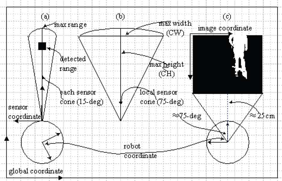
(a) The kinematical transformation; (b) Local sensor cone; (c) Image frame transformation

Fig. 3.

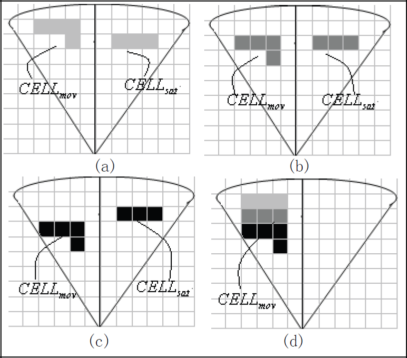
A sequence of time-variant maps describing a simple environment, different gray levels represent the age of observation, darker ones corresponding to the more recent

Fig. 3.

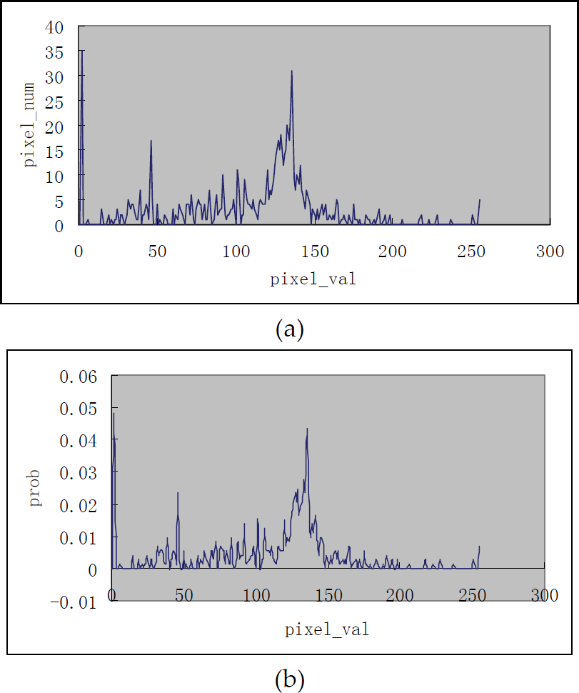
Intensity histogram of a particular pixel over 15min (a) in a dynamic indoor environment and corresponding emission model (b)

4.2. Detecting Moving Objects

Due to the noise and uncertainty inherently in the sonar sensors, to keep false moving object detection events at a low rate, we do not track single cells that are apparently moving, but the cluster ensembles of coherently moving cells into distinct objects even though which may be only part of certain object. The cell clustering algorithm here is temporarily simple: to check the adjacent cells, if occupied, they are considered as the same class, otherwise considered as different ones. In this work, we use Sonar Temporal Difference with a sequence of time-variant maps to detect moving objects. We consider the set of cells in TVM_t which carry a time tag t (occupied at time t) and test whether the corresponding cells in TVM_t-1 were occupied too, i.e., carry a time tag t-1. If corresponding cells in TVM_t, TVM_t-1 carry time tags t and t-1, respectively, then we interpret the spatial region circumscribed by these cells occupied by a stationary object CELL_sat. If, however, the cells in TVM_t-1 carry a time tag different from t-1 or no time tag at all, then the occupation of the cells in TVM_t must be due to a moving object CELL_mov. If it is detected as a stationary object, we filter this object out of the time-variant map by simply freeing the corresponding occupied cells, while the moving objects stay left in the time-variant map. Fig. 3d shows the result of Sonar Temporal Difference based on the sequence of time-variant maps shown in Fig. 3a–3c. Note that here we consider only the two most recent maps, TVM_t and TVM_t-1, for detecting moving objects. This limits our motion detection resolution, since objects that move very slowly as compared to the sensor sampling rate will not be detected as moving. This problem can be alleviated by selecting an appropriate value of n (n = τ / t) and by using Bayesian update rule which can update the dynamic object states in fuzzy-tuned grid-based map. The outline of Sonar Temporal Difference algorithm is shown in pseudo-code in Table 1.

Table 1.
Sonar Temporal Difference Algorithm

Begin Algorithm MotionDetection_STD

FOR each cell class cc_x, t representing an object x in TVM_t

FOR each cell c_i, t in cc_x, t

FOR each corresponding cell c_i, t-1, …, c_i, t-k, …, c_i, t-n in TVM_t-1, …, TVM_t-k, …, TVM_t-n

IF c_i, t-k carries a time tag t-k THEN

c_i is occupied by a stationary object

ELSE

c_i is occupied by a moving object

IF majority of cells c_i, t in cc_x, t is moving THEN

cell class cc_x, t is moving, i.e. CELL_mov

ELSE

cell class cc_x, t is stationary, i.e. CELL_sat

IF CELL_sat THEN

free the corresponding occupied cells

ELSE IF CELL_mov THEN

do nothing

End Algorithm

5. Statistical Background Subtraction (SBS)

A common method to track motion in image sequences is background subtraction between an estimate of the image without moving objects and the current image. Previous researcher (Rittscher, J. et al 2000; Ren Y. et al 2003; Rowe S. & Blake, A. 1996) have shown that the disruption can be somewhat suppressed by using statistical model of background in image-subtraction to find motion. Here, we also adopt a statistical method to model the background: a 3-class mixture of Gaussians, which is learned by using Expectation-Maximization (EM) algorithm (Dempster, A. P. et al 1977). We consider the intensity values of a particular pixel over time as an independent statistical process called “pixel process” (refer to Fig. 3). In a structured indoor environment, due to the lighting changes, scene changes, and moving objects, the distribution of each pixel is fitted with multiple Gaussians. Since illumination is one of the important components in indoor environments, it is necessary to discriminate the shadows from background and foreground. Therefore, we adopt a 3-class mixture of Gaussians to model the pixel process. Since it is hard to estimate the distribution of foreground along the image sequence, we adopt uniform distribution to represent it.

\begin{aligned} p (z) & = ω_{F} * p_{F} (z) + ω_{B} * p_{B} (z) + ω_{s} * p_{s} (z) \\ = ω_{F} * \frac{1}{R} + ω_{B} * \frac{1}{\sqrt{2 π σ_{x_{B}}}} \exp (- \frac{(z - μ_{x_{B}})^{2}}{{2 σ_{x_{B}}}^{2}}) \\ + ω_{s} * \frac{1}{\sqrt{2 π σ_{x_{s}}}} \exp (- \frac{(z - μ_{x_{s}})^{2}}{{2 σ_{x_{s}}}^{2}}) \end{aligned}

(4)

where

ωF,ωB,ωS: Weights of the three distributions in the mixture, respectively.

μxB, μxS: Means of the two Gaussians in the mixture, respectively.

ςxB, ςxS: Standard deviations of the two Gaussians in the mixture, respectively.

R: Parameter of the uniform distribution in the mixture, decided by the valid range of the intensity value. Usually it is 256.

In the learning stage, we use EM algorithm to estimate the model parameters by given a training sequence like (Rowe S. & Blake, A. 1996). It should be noted that EM algorithm is not guaranteed to find global maximum and very sensitive to the starting point. That is, the algorithm will not converge quickly and fail to fit the distribution properly, if given a poor initial estimate of the distribution. In our work, we empirically determine the initialization similar with (Rittscher, J. et al 2000).

5.1. Motion Detection

In our work, when new frame is available, we have to compensate the sensor motion in order to use background subtraction to detect foreground objects. That is, we map each pixel in current frame xc into background frame. Due to the errors in feature localization, motion estimation etc., this map process is not very accurate. So, at best, we predicate a position ○_B, i.e. Tx_F = α○_B, where T is the transition matrix for background motion compensation and a is a nonzero scalar. We use iterative closed point (ICP) algorithm to determine T : Using a reasonably good initial guess of the relative transformation, a set of salient landmarks are chosen from front image (i.e. current frame) and background.

L_{F} = {l_{F, i}, i = 1, 2, \dots, n}, L_{B} = {l_{B, i}, i = 1, 2, \dots, n} .

l_{F, i} and l_{B, i} are the corresponding landmarks in current and background frame respectively. The better estimate of the relative transformation T is iterated by least-square-estimation (LSE) method. Because the motion compensation is not accurate, that is ○_B will not definitely the corresponding pixel xF, in order to comprise this approximate alignment, we adopt another Gaussian model called alignment Gaussian model (AGM) (Fig. 4), which centers at ○_B with covariance matrix Σ in a validation region $ℜ_{{\hat{x}}_{B}}$ similar with SGD in (Ren Y. et al 2003).

p (x_{B} ∣ {\hat{x}}_{B}) = \frac{1}{2 π | \sum |^{1 / 2}} \exp (- \frac{1}{2} (x_{B} - {\hat{x}}_{B})^{T} \sum^{- 1} (x_{B} - {\hat{x}}_{B}))

(5)

ℜ_{\hat{x} B} = {x_{B} : D_{x B, \hat{x} B} \leq λ^{_}}

(6)

D_{x B, \hat{x} B} = (x_{B} - {\hat{x}}_{B})^{T} \sum^{- 1} (x_{B} - \hat{x} B)

(7)

Σ = β \hat{Σ}

(8)

\hat{Σ} = \frac{1}{n} \sum_{i = 1}^{n} (l_{F, i} - l_{F, i}^{'}) (l_{F, i} - l_{F, i}^{'})^{T}

(9)

α l_{F, i}^{'} = T l_{B, i}

(10)

Fig. 4.

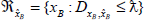
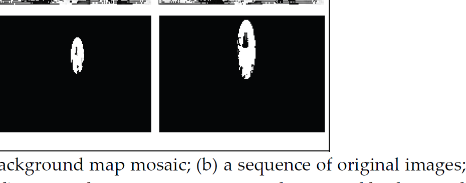
Illustration of xB, xF with their AGMs

Σ is important for determining the size of AGM and will be different from pixel to pixel. But here for computational simplicity, we assume it is constant and estimated by Eq. (8). With $\hat{Σ}$ is estimated, as coefficient β increases, the size of AGM increase and different results of the detection are obtained accordingly. In our work, since the environment is structured, we select a proper β empirically. Therefore, for a particular pixel in current frame xF, there is a corresponding AGM in the background map. If XF belongs to any of the background Gaussians of its AGM, it is labeled as background. If no corresponding background distribution can be found in its AGM, the pixel xF is regarded as foreground.

5.2. Background Update

Everything above works well while the background is adequately updated. But this is not easy for a moving background, especially when there is an occlusion and/or uncovered background. Here we use the similar approach with (Ren, Y. et al 2003) to update nonstationary background. We briefly report the algorithm as Table 2. For details, please refer to (Ren Y. et al 2003). And a preliminary experimental result of proposed algorithm is shown in Fig. 5.

Table 2.
Background Update Algorithm

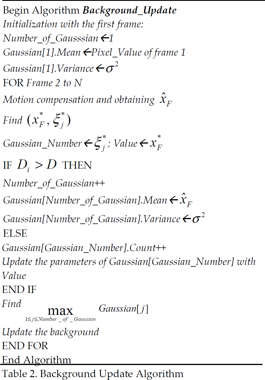
Begin Algorithm Background_Update

Initialization with the first frame:

Number_of_Gausssian ←1

Gaussian[1]Mean ←Pixel_Value of frame 1

Gaussian[1]. Variance ← ς²

FOR Frame 2 to N

Motion compensation and obtaining ○_F

Find ( $(x_{F}^{}, ξ_{j}^{})$ )

Gaussian_Number $ξ_{j}^{}$ Value $x_{F}^{}$

IF D_i > D THEN

Number_of_Gaussian++

Gaussian[Number_of_Gaussian]Mean ←○_F

Gaussian[Number_of_Gaussian]. Variance ←ς²

ELSE

Gaussian[Gaussian_Number].Count++

Update the parameters of Gaussian[Gaussian_Number] with Value

END IF

Find

$max_{1 \leq j \leq N u m b e r_o f_G a u s s i a n} G a u s s i a n [j]$

Update the background

END FOR

End Algorithm

Fig. 5.

Motion detection with nonstationary background. (a) background map mosaic; (b) a sequence of original images; (c) motion detection using common background subtraction; (d) motion detection using proposed statistical background subtraction

6. Fuzzy-Tuned Integration (FTI)

After detecting moving objects respectively by the sonar sensors and the uncalibrated camera, we need to integrate these two different sources into the result global map with filtering out the spurious objects. However, since the camera is uncalibrated, that is, lack of the inter-parameters of the camera, we can not know the precise distance measurement from images, additionally, the sonar is also not very accurate because of the uncertainty in radial and angular, therefore, we can not directly use traditional multisensor fusion (Castellanos, J. A. et al 2001) which requires precise sensor-sensor calibration to integrate these two detection results into a common reference frame.

In order to achieve a reliable integration, in this paper, we propose Fuzzy-Tuned Integration (FTI) algorithm to find out the spurious objects in the fuzzy-tuned grid-based map, which needs two necessary parameters: location and size of the spurious objects in the resulting map, and then filter them out. To design this fuzzy system, we first define the input variables and output variables as follows:

Input Variables

B_Centroid(x, y): The centroid of BLOB_mov in robot frame.

C_Centroid(x, y): The centroid of CELL_mov in robot frame.

B_Size: The size of the BLOB_mov in vision frame in number of pixels.

C_Size: The size of the CELL_mov in grid-based map in number of grids.

Output Variables

O_Centroid (x, y): The centroid of update region in robot frames.

O_Size: The size of update region in number of grids.

Tables 3–5 show the fuzzy rule-base for tuning the output variables, and the membership functions and linguistic states are in Fig. 6. where

Fig. 6.

Membership functions and output consequence fuzzy sets corresponding to fuzzy rule base in Tab. 3–5.

Table 3.

Fuzzy rule table corresponding to O_Centroid.x

		B_Centroid.x
		VS	S	M	L	VL
C_Centroid.x	VS	VS	S	S	M	M
	S	VS	S	M	M	L
	M	S	S	M	L	L
	L	M	M	M	L	VL
	VL	L	M	L	L	VL

Table 4.

Fuzzy rule table corresponding to O_Centroid.y

		B_Centroid.y
		NB	NS	Z	PS	PB
C_Centroid.y	NB	NB	NS	NS	Z	Z
	NS	NB	NS	Z	Z	PS
	Z	NS	NS	Z	PS	PS
	PS	Z	Z	Z	PS	PB
	PB	PS	Z	PS	PS	PB

Table 5.

Fuzzy rule table corresponding to O_Size

		B_Size
		VS	S	M	L	VL
C_Size	VS	VS	S	S	L	VL
	S	S	S	M	L	VL
	M	M	M	M	L	VL
	L	L	L	L	L	VL
	VL	VL	VL	VL	VL	VL

IW: The image width (in our experiment, this value is fixed at 160 pixels)

IH: The image height (in our experiment, this value is fixed at 120 pixels)

CW: The maximum width of the local sensor cone

CH: The maximum height or range in the local sensor cone

Note that in this fuzzy system, the image coordinate has been transformed into the robot frame according to Fig. 2.

Everything explained above works fine under the assumption that motion correspondence problem has been well solved, that is the moving object pair respectively detected by sonar sensor and un-calibrated camera already finely associated to each other. However, this problem can seriously damage the resulting map if the motion correspondence is not well done. In computer vision literature, there already exist many approaches to solve this problem, such as track-splitting joint likelihood, multiple hypothesis algorithm etc. Cox has a good review to this problem in (Cox, I. J. 1993). In our work, we use the Nearest-Neighbor algorithm to solve the detected moving object association. The nearest-neighbor algorithm is the simplest suboptimal data-association algorithm, which assumes that each measurement originates from the closest corresponding feature, in our experiment, where closest is defined using the Euclidean distance of the centroids of the detected moving objects formulated by Eq. 11. Note that B_Centroid(x, y) and C_Centroid (x, y) were transformed into the same coordinate frame according to Fig. 2.

D I S T = | B_C e n t r o i d (x, y) - C_C e n t r o i d (x, y) |

(11)

Since our experiment is performed in the indoor dynamic environment which is structured and also has not many moving objects to detect and track, hence the nearest-neighbor algorithm can satisfy our need. So, our fuzzy-tuned integration works only when we find there exist corresponding moving objects, i.e. only when DIST > ς_correspond, where ς _correspond is motion correspondence threshold obtained by trial and error. The whole outline of proposed fuzzy-tuned integration algorithm is shown in pseudo-code in Table 6.

Table 6.

Fuzzy-tuned integration algorithm

Begin Algorithm FuzzyTunedIntegration

FOR each detected moving objects by camera in image, i.e.

B_Centroid (x, y)

FOR each detected moving objects by sonar in grid map, i.e.

C_Centroid(x, y)

Computing DIST

IF DIST > ς_correspond THEN

Incorporating the results of two types of motion detection by using fuzzy-tuned integration and filter these spurious objects out of the grid-based map

ELSE

Do nothing

Improving the resulting grid-based map by freeing much isolated occupied grids

Waiting for next map update cycle

End Algorithm

7. Simulation and Experimental Results

7.1. Simulation Study

In this simulation study, we try to illustrate that the Bayesian update rule used in our proposed algorithm is capable to update dynamic object states like slow relocation. To explain the results more easily, we only consider the one-dimension environment and assume that the sensor measurement is r_i and there is a dynamic obstacle which changes its location over time. The motion profile of the object is shown as follows:

Location 1: Obstacle is stayed 1m away from the sensor. i.e. {r_i =1m, i =1, 2,…, 8}

Location 2: Obstacle is moved to 1.6m away from the sensor. i.e. {r_i =1.6m, i =9, 10,…, 16}

Location 3: Obstacle is moved to 0.5m away from the sensor. i.e. {r_i =0.5m, i =17, 18, 19,…}

The profiles of occupancy probabilities corresponding to 7^th, 8^th, 15^th, 16^th, 23^rd, 24^th readings for our proposed algorithm are shown in Fig. 7. From this Fig., we can observe that our algorithm can provide good estimate of the obstacle position when is moved from Location 1 to Location 2 and from Location 2 to Location 3. Therefore, it can be concluded that this algorithm is suitable for updating the states of dynamic objects.

Fig. 7.

The result of the algorithm to update the state of dynamic object

7.2. Experimental Study

The goal of the experiment is to illustrate that fuzzy integration of two detection techniques, STD and SBS, into the mapping process leads to a better global resulting map since spurious objects were filtered out. The experiment was carried out on the Pioneer 1 robot in the corridor at HKPU. The robot is equipped with one uncalibrated camera with a fixed angle and seven sonar sensors, five locating front, separated by 15-degree each, and two locating at each side. The driving mechanism is by means of 2 reversible DC motors with wheel encoders to update the location by dead reckoning. The software is written in C language and Saphira software (ActivMedia 1998) with API libraries has been used to obtain the sonar data and to perform the localization to estimate the current position and orientation of the robot. The navigation is not autonomous in the present implementation. The robot is manually navigated to predefined locations such that to avoid the dead reckoning error due to slip. The sonar sensors were measurements in a range up to 3 meters around the robot which were considered relevant for mapping, and the maximum distance of the camera visual zone we concerned in this experiment is also around 3 meters which can highly improve the quality of the fuzzy-tuned integration. Fig. 8 shows the hand-measured model of this environment to be mapped.

Fig. 8.

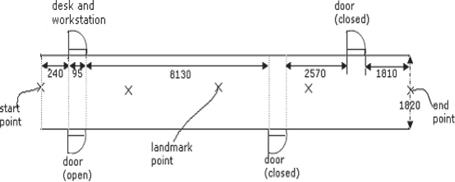
Hand-measured model of the corridor in HKPU

During mapping, there were several (up to three) people walking in front of the robot. Fig. 9 shows the robot during the mapping process. Fig. 10a shows the raw range sonar measurements which were obtained by the robot and the map obtained without people filtering. And the resulting map obtained with our proposed algorithm is shown in Fig. 10b. Both maps have a resolution of 50mm per cell. As seen from Fig. 10a, there are a many cells in the resulting grid map, which have a high occupancy probability since people covered the corresponding area while the robot was mapping the environment. If, however, we use the proposed algorithm and filter out the most of moving objects (here is people), the effect of the people is seriously reduced in the resulting map (see Fig. 10b).

Fig. 9.

Pioneer 1 mobile robot is mapping a dynamic corridor environment.

Fig. 10.

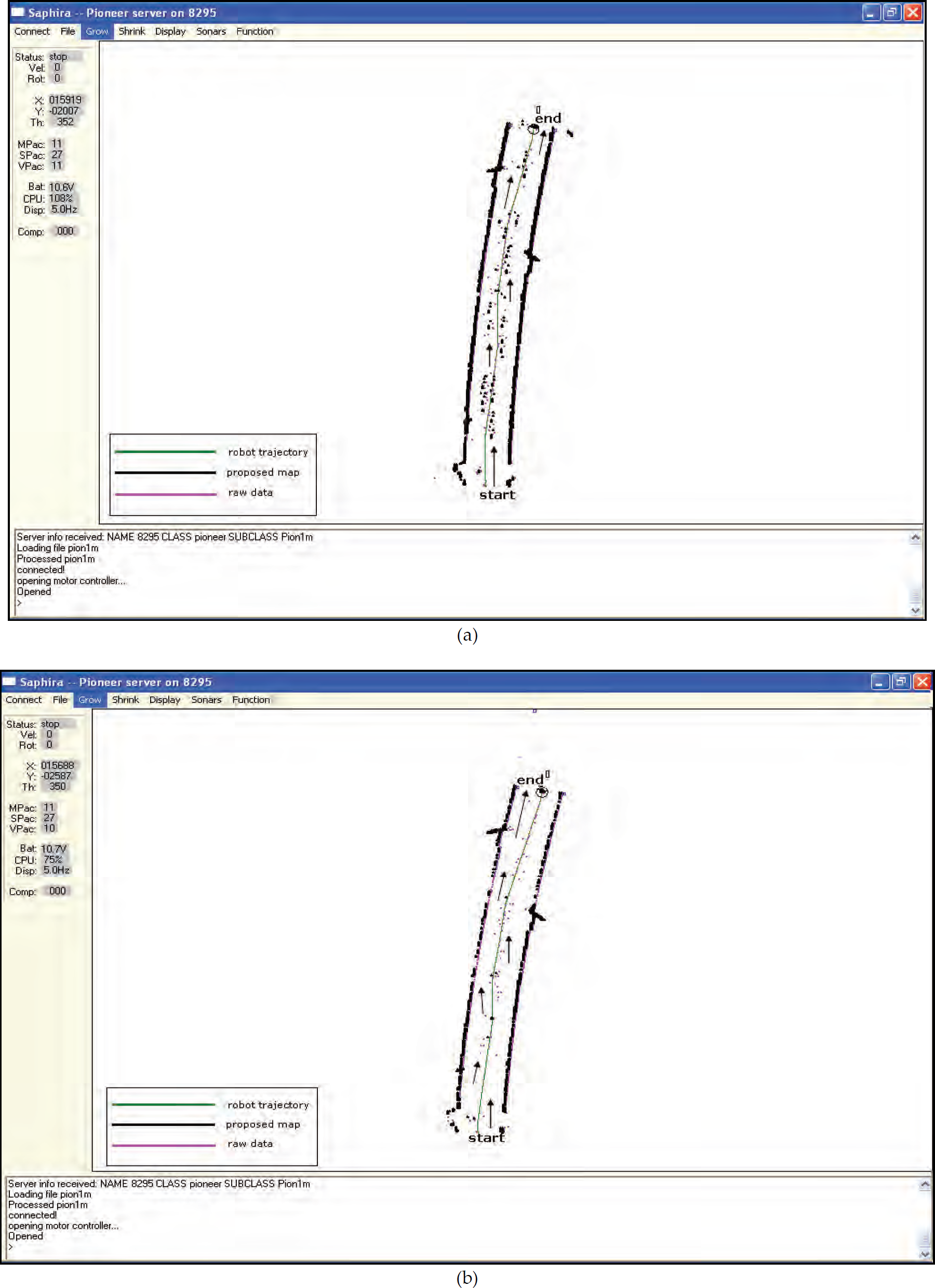
(a) Fuzzy-tuned grid-based map without filtering out moving objects; (b) Resulting map of proposed algorithm

Therefore, as see from Fig. 10(a–b), the algorithm is more reliable for mapping in dynamic environments than fuzzy-tuned grid-based mapping method as well as traditional mapping methods.

Note that sine the robot has only seven sonar sensors, five located forward, separated by 15-degree each and two at both sides. Additionally our camera faces forward at a fixed angle. Thus both sensors only have a limited measurement zone (about 75-degree). Considering these limits, we assume d that people only walked in front of the robot during the experiment. And since localization problem was temporarily ignored in this paper and we used odemetric measurements to localize the robot's position with predefined landmarks, there must be some dead reckoning errors. Thus the resulting map was not rectangular compared with the hand-measured map. The localization problem will be addressed in future work.

8. Conclusions

In this paper, we have presented a new solution to map structured indoor dynamic environments that incorporates motion tracking into mapping process. The two methods used in motion tracking are sonar temporal difference and statistical background subtraction methods. The former is constructed by monitoring a sequence of temporal local maps. The latter is achieved based on sufficient background update with a 3-class mixture of Gaussians. After detecting the dynamic entries, due to no accurate transformation between image plane and robot local frame, we applied a fuzzy system to integrate these two methods to filter out the spurious objects from the resulting map. We demonstrated that detection of dynamic entries can benefit the maping process. Simulation and experimental results show the capability of the proposed algorithm.

As the main focus of this work is the fuzzy integration of motion detection into mapping, localization temporarily is not an issue. As the future work, we will incorporate localization into this work to solve the problem of simultaneous localization and mapping (SLAM) in dynamic environments. We also plan to extend this work to deal with more complex environments. We will investigate alternative algorithms of detecting moving objects to improve the accuracy and efficiency of the motion detection and accordingly improve the resulting map.

References

ActivMedia (1998). Saphira Manual, Version 6.1e.

Andrade-Cetto

& Sanfeliu

(2002). Concurrent map building and localization on indoor dynamic environments, International Journal on Pattern Recognition and Artificial Intelligence. 16: 361–374.

Anguelov

Biswas

Koller

Limketkai

Sanner

& Thrun

(2002). Learning hierarchical object maps of non-stationary environments with mobile robots, In Proceedings of the 17th Annual Conference on Uncertainty in AI (UAI).

Biswas

Limketkai

Sanner

& Thrun

(2002). Towards object mapping in non-stationary environments with mobile robots, In Proceedings of the Conference on Intelligent Robots and Systems (IROS), Lausanne, Switzerland.

Burgard

Cremers

A. B.

Fox

Hähnel

Lakemeyer

Schulz

Steiner

& Thrun

(1999). Experiences with an interactive museum tour-guide robot, Artificial Intelligence, 114(1–2):3–55.13.

Castellanos

J.A.

Neira

& Tarós

J.D.

(2001). Multisensor fusion for simultaneous localization and map building, IEEE Robotics and Automation, 17(6).

Chow

K.M.

Rad

A.B.

& Ip

Y.L.

(2002). Enhancement of probabilistic grid-based map for mobile robot applications, Journal of Intelligent and Robotic Systems, 34 (2): 155–174.

Cox

I.J.

(1993). A review of statistical data association techniques for motion correspondence, International Journal of Computer Vision, 10(1): 53–66.

Dempster

A. P.

Laird

N. M.

& Rubin

D. B.

(1977). Maximum likelihood from incomplete data via the EM algorithm. Journal of the Royal Statistical SocietyB, 39(1):1–38.

10.

Elfes

(1989). Using occupancy grids for mobile robot perception and navigation, IEEE Computer 22(6):46–57.

11.

Fox

Burgard

& Thrun

(1999). Markov localization for mobile robots in dynamic environments, Journal of Artificial Intelligence Research, 11:391–427.

12.

Hähnel

Schulz

& Burgard:

(2003). Mobile robot mapping in populated environments, Advanced Robotics, 17 (7): 579–598.

13.

Han

Cha

Hong

& Hahn

(2001). Tracking of a moving object using sonar sensors based on a virtual sonar image, Robotics and Autonomous Systems, 36: 11–19.

14.

Y. L.

Rad

A. B.

Chow

K. M.

& Wong

Y. K.

(2002). Segment-based map building using enhanced adaptive fuzzy clustering algorithm for mobile robot applications, Journal of Intelligent and Robotic Systems, 35(3): 221–245.

15.

Bosse

Newman

P. M.

Leonard

J. J.

& Teller

(2004). SLAM in Large-scale Cyclic Environments using the Atlas Framework. International Journal of Robotics Research, 23(12): 1113–1139.

16.

Montemerlo

Whittaker

& Thrun

(2002a). Conditional particle filters for simultaneous mobile robot localization and people-tracking, In IEEE International Conference on Robotics and Automation (ICRA), Washington, DC.

17.

Montemerlo

Thrun

Koller

& Wegbreit

(2002b). FastSLAM: A factored solution to the simultaneous localization and mapping problem, in: Proc. AAAI National Conference on Artificial Intelligence, 593–598.

18.

Prassler

& Scholz

(2000). Tracking multiple moving objects for real-time robot navigation, Autonomous Robots, 8: 105–116.

19.

Rittscher

Kato

Joga

& Blake

(2000). A probabilistic background model for tracking, Proceedings of the European Conference on Computer Vision, 336–351.

20.

Ren

Chua

C. S.

& Ho

Y.K.

(2003). Motion detection with nonstationary background. Machine Vision and Application, 13: 332–343.

21.

Remolina

& Kuipers

(2004). Towards a general theory of topological maps, Artificial Intelligence, 152 : 47–104.

22.

Rowe

& Blake

(1996). Statistical mosaic for tracking. Image Vision Comput 14:549–564.

23.

Thrun

(1998a). Learning metric-topological maps for indoor mobile robot navigation, Artificial Intelligence, 99(1):21–71.

24.

Thrun

Fox

& Burgard

(1998b). A probabilistic approach to concurrent mapping and localization for mobile robots, Machine Learning, 31:29–53.

25.

Thrun

Beetz

Bennewitz

Burgard

Cremers

A. B.

Dellaert

Fox

Hähnel

Rosenberg

Roy

Schulte

& Schulz

(2000). Probabilistic algorithms and the interactive museum tour-guide robot Minerva, Journal of Robotics Research, 19(11).

26.

Thrun

(2001a). A probabilistic online mapping algorithm for teams of mobile robots, International Journal of Robotics Research, 20(5):335–363.

27.

Thrun

Fox

Burgard

& Dellaert

(2001b). Robust Monte Carlo Localization for mobile robots, Artificial Intelligence, 128(1–2).

28.

Thrun

(2002). Robotic mapping: A survey, Technical Report CMU-CS-02-111, CMU.

29.

Schulz

& Burgard

(2001). Probabilistic state estimation of dynamic objects with a moving mobile robot, Robotics and Autonomous Systems, 34 (2–3): 107–115.

30.

Schulz

Burgard

Fox

& Cremers

A.B.

(2003). People tracking with a mobile robot using sample-based joint probabilistic data association filters, International Journal of Robotics Research, 22 (2).

31.

Wang

C.-C.

(2004). Simultaneous localization, mapping and moving object tracking, PhD thesis, Carnegie Mellon University.

32.

Wang

L. X.

(1997). A course in fuzzy systems and control, Prentice-Hall International Inc.

33.

Wolf

& Sukhatme

(2005). Mobile Robot Simultaneous Localization and Mapping in Dynamic Environments, Autonomous Robots, 19(1): 53–65.

A New Solution to Map Dynamic Indoor Environments

Abstract

Keywords

1. Introduction

2. Related Work

3. Fuzzy System and Fuzzy-Tuned Grid-Based Map (FTGBM)

3.1. Notation and Definition of Fuzzy System

4.1. Time-Variant Map (TVM)

7.1. Simulation Study

References