Exploration and Navigation for Mobile Robots With Perceptual Limitations

Abstract

To learn a map of an environment a mobile robot has to explore its workspace using its sensors. Sensors are noisy and have perceptual limitations that must be considered while learning a map. This paper considers a mobile robot with sensor perceptual limitations and introduces a new method for exploring and navigating autonomously in indoor environments. To minimize the risk of collisions as well as to not exceed the range of sensors, we introduce the concept of a travel space as a way to associate costs to grid cells of the map, based on distances to obstacles. During exploration the mobile robot minimizes its movements, including rotations, to reach the nearest unexplored region of the environment, using a dynamic programming algorithm. Once the exploration ends, the travel space is used to form a roadmap, a net of safe roads that the mobile robot can use for navigation. These exploration and navigation method are tested using a simulated and a real mobile robot with promising results.

1. Introduction

This paper introduces an exploration approach for an indoor mobile robot using its sensors, to learn a Probabilistic Grid-based Map (PGM) (Elfes, A., 1989; Moravec, H. P., 1988; Thrun, S., 1998a) of an environment. A PGM is a two dimensional map where the environment is divided in square regions or cells of the same size that have occupancy probabilities associated to them. The map learned is commonly used by a mobile robot for navigation while it does a high level task. Research on exploration strategies has developed two general approaches: reactive and model based (Lee, D., 1996). By far the most widely-used exploration strategy in reactive robotics is wall following. Model based strategies vary with the type of model being used, but they are based on the same underlying idea: go to the least-explored region (Lee, D., 1996).

During the exploration of the environment, the robot movements are typically measured by an odometer. However, the odometer introduces errors that accumulate over time. In order to build useful maps, odometric errors have to be reduced or corrected, usually using other sensors. Given the perceptual limitations and accuracy of sensors, odometric errors can not always be reduced. Typically sensors like sonars and cameras can detect obstacles within a range of a few meters and their accuracy decreases with the distance to obstacles. The reduction of odometric errors in this case is known as the position tracking problem or the local localization problem.

There are several successful localization methods that can estimate the robot's position using its sensors. However, most localization methods fail when the sensors of the robot are beyond its perceptual capability (Roy et al, 1999) (i.e., the robot is too far from obstacles).

This paper introduces a novel approach to explore a static indoor environment. The idea is to reach the nearest unexplored grid cell minimizing a travel cost. The travel cost takes into account the movements of the robot (including rotations) and the perceptual limitations of the sensors, and tries to maintain a fixed distance to obstacles while the robot is moving, like a wall following strategy (Lumelsky, V. J. & Stepanov, 1987). In contrast to other methods, this approach considers rotations of the robot besides translations.

The concept of a (travel space) is introduced to assign costs to grid cells, based on distance to obstacles. An optimal motion policy for the robot is computed using a dynamic programming algorithm, a modified version of value iteration (McKerrow, P. J., 1991) that includes the orientation of the robot in the representation of the states. The optimal motion policy considers: cost of grid cells, movements of the robot (translations and rotations) and the nearest unexplored cells.

Once the map is complete, the travel space is also used to obtain an efficient navigation technique based on the same dynamic programming algorithm. The idea is to reduce the number of free cells to be processed, significantly reducing the computational cost. A road map (Latombe, J-C., 1991) is built upon the travel space, where only the cells of the road map are included in the dynamic programming algorithm for navigation.

These ideas have been tested using a mobile robot simulator and a real mobile robot in indoor environments. Experiments show that the robot tries to keep a safe distance to obstacles, minimizing the risk of collisions with obstacles and of getting lost, and it also reduces the number of movements (including rotations) while it is exploring an environment and consequently reduces its odometric errors. This results in more accurate maps.

In (Roy et al, 1999), a coastal navigation method similar to our navigation approach is described, once a PGM has been built. Each cell in the map contains a notion of information content available at this point in the map, which corresponds to the ability of the robot to localize itself. The information content is based on the concept of entropy and some assumptions are considered to reduce the complexity of the method. Our approach generates a similar form of coastal navigation with a simpler and more efficient method. The incremental algorithm developed in this paper also fits the time requirements for the exploration task.

In another related work (Thrun, S., 1998b), the probability of occupancy of a grid cell is used as a cost associated to the cell. The motion policy, given by value iteration, does not consider rotations of the robot and needs to be post-processed in order to keep the robot near to the center of narrow passages (but they do not describe how to do that). In our approach there is no need to modify the policy given by the value iteration algorithm. The local guides, in the form of costs, are inside the value iteration algorithm, so the policy is optimal given the costs associated to cells and the cost to move (translation and rotation) to an adjacent cell.

The remainder of the paper is organized as follows. Section 2 describes the proposed exploration approach. Section 3 describes the navigation method, once the map has been built. Section 4 presents experimental results using a mobile robot simulator and a real mobile robot. The experiments are performed using a system build upon the ideas for sensor data fusion and position tracking described in (Romero, I., Morales, E., & Sucar, E., 2000). Finally, section 5 is devoted to conclusions and future work.

2. Exploration

Given that robotic sensors only cover a small area around it and they can not see through walls, the robot has to explore the environment to build a complete map. For this it uses its sensors and moves to different locations, until all areas are covered. The process we use to build a probabilistic grid map does the following general steps:

Process the readings taken by all the sensors and update the probability of occupancy of the cells in the PGM (Sensor Data Fusion Step).

Update the travel space accordingly considering the changes in the PGM.

Choose the next movement using value iteration. If all the grid cells accessible to the robot are explored then the map is complete. Otherwise all free cells have the optimal movement to reach the nearest unexplored cell.

Execute the movement of the cell associated with the robot current position.

Get readings from the sensors and correct odometric error (Position Tracking Step).

Go to the first step.

Next we review steps 1 to 5, with steps 2 and 3 (the key steps of our approach) covered in more detail.

The general idea for exploration is to move the robot on a minimum-cost path to the nearest unexplored grid cell (Thrun, S., 1998b). The minimum-cost path is computed using value iteration, a popular dynamic programming algorithm. In (Thrun, S., 1998b) the cost for traversing a grid cell is determined by its occupancy probability, while in (McKerrow, P. J., 1991) the cost is determined by the distance between cells (see Chapter 8 in (Lee, D., 1996)).

This paper proposes a new approach that combines local search strategies within a modified version of value iteration described in (McKerrow, P. J., 1991). When the robot starts to build a map, all the cells have the same probability of occupancy, P(O)=0.5. A cell is considered unexplored, when its occupancy probability is in an interval (close to 0.5) defined by two constants [Pe_min, Pe_max] (Pe_min < 0.5 < Pe_max) and explored otherwise.

In an alternative approach (Thrun, S., 1998b), a cell is considered explored when it has been updated at least once. That approach, however, does not work well when there are specular surfaces (i.e., using ultrasonic range sensors) in the environment, since multiple measurements are normally required to get reliable estimates for the probability of occupancy of a cell.

Cells are defined as free or occupied. A cell is considered occupied when its P(O) reaches a threshold value Po_max and continues to be occupied while its P(O) does not fall below a threshold value Po_min (where Po_min < Po_max). It is considered free in other case. This mechanism prevents changes in the state of occupancy of a cell by small probability changes. We assume that Pe_max < Po_min, so an unexplored cell is also a free cell. In this way, the PGM becomes a binary map when cells are classified as occupied or free. This binary map will be called occupied-free map.

In this work, a cylindrical (circular base) robot is considered, so the configuration space (c-space) (Latombe, J-C., 1991) can be computed by growing the occupied cells by the radius of the robot. In fact, the c-space is extended to form a travel space. The idea behind the travel space is to define a way to control the exploration by a kind of wall following strategy. Wall following is a local method that has been used to navigate robots in indoor environments, but unfortunately it can easily get trapped in loops (Lee, D., 1996). The travel space together with a dynamic programming technique has the advantages of both, local and global strategies: robustness and completeness.

2.1. Step 1: Sensor Data Fusion

In this work it is considered that the robot has three types of sensors:

Ultrasonic range sensors. In this case, let P(O_s) be the occupancy probability of the cell (x, y) detected only by sonars.

Laser range sensors. In the same way, let P(O_l) be the occupancy probability detected only by this type of sensors.

Maneuverability. The mere fact that a robot moves to a location (x, y) makes it unlikely that this location is occupied. Let P(O_m) be the occupancy probability detected by this type of sensor.

We extend the idea of sonar data fusion given in (Howard, H. & Kitchen, L., 1996) to fuse data from sensors of different types. We consider a cell as occupied if it is detected occupied by at least one sensor. In this way, the probability that a given cell is occupied can be estimated using a logical OR operation among the occupancy states detected by each type of sensor:

$$P(O)=P(O_{\mathrm{s}}OR{O}_{l}OR{O}_{\mathrm{m}})$$

(1)

To expand the right hand side of (1), it is assumed that the events O_s, O_l, and O_m are statistically independent. This assumption make sense if we consider that the environment has obstacles like transparent walls (detected by sonars but not by laser range sensors) or thin sticks (detected by laser range sensors but not by sonars). With this assumption, and after some algebra, equation (1) becomes:

$$P(O)=1-\prod _{i=s,l,m}(1-P(O_i))$$

(2)

This expression can be used to compute the probability that a cell is occupied once we have determined the probability that a cell is occupied by each type of sensor. The prior probabilities, P(O), are initially set to 0.5 to indicate ignorance. This implies that the prior probabilities for the variables associated to each type of sensor i (i=s, l, m) for every cell are given by: P_prior(O_i)=1 - (0.5)^1/3. Further details of this step are given in (Romero, I., Morales, E., & Sucar, E., 2000).

2.2. Step 2: Update the travel space

Consider the travel space due to a single real occupied cell in the occupied-free map (see Figure 1). The travel space splits the cells of the occupied-free map in four categories:

Occupied cells. These cells are inside the circle given by the radius of the robot (as in the c-space) with center in the real occupied cell. After this expansion, the robot is considered as a single cell.

Warning cells. Cells close to an occupied cell. Let D_w be the maximum distance between a cell of this type and its closest real occupied cell. These cells are called warning cells because their purpose is to warn the robot about its closeness to an obstacle. The value of D_w takes into account the perceptual limitations of the sensors. This value can be adjusted for more or less reliable sensors or for different environments (e.g., with many windows), changing the travel space.

Travel cells. Cells close to a warning cell. Let D_t be the maximum distance between a cell of this type and its closest real occupied cell. These cells are called travel cells because their purpose is to suggest to the robot a path to follow.

Far cells. Any free cell (in the occupied-free map) that is not a warning or a travel cell.

Fig. 1.

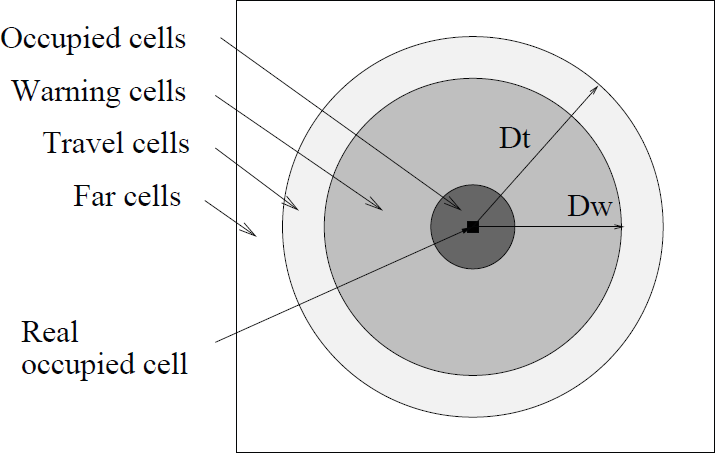
Travel space due to a single occupied cell.

The idea to suggest safe paths to the robot is to assign a high cost to far cells, a low cost to travel cells and higher costs to warning cells. In order to assign higher costs to warning cells closer to obstacles, each warning cell must record, besides its type, the distance to the nearest occupied cell, denoted by d_min. For travel and far cells it is enough to record the cell's type. The travel space can be computed incrementally after each change of state of a cell in the occupied-free map, while the robot is exploring the environment. The algorithm is as follows:

Initialization. Let all free cells in the travel space be of type far.

If there is a change from free to occupied cell, do:

Grow the occupied cell by a radius of the robot. Assign the type occupied to the cells in the circle.

Using a larger circle, compute the warning cells (see Fig. 1). For each of these cells, let d be the distance from the cell to the center of the circle, and t_old be the type of cell previously assigned to the cell. If (t_old in {travel, far}) or ((t_old = warning) and (d < d_min)) then assign the type warning to the cell and set d_min = d. The size of the circle depends on the perceptual limitations of the sensors.

Using a larger circle, compute the travel cells (see Fig. 1). For each of these cells, let t_old be the type of cell previously assigned to the cell. If (t_old = far) then assign the type travel to the cell.

If there is a change from occupied to free cell, do:

Using a circle of radius D_t, equal to the outer circle used to compute the travel cells, assign the type far to all the cells under the circle. In other words, it cleans the effect of the previous occupied cell.

Consider a circle of radius 2D_t. For each occupied cell inside this circle in the occupied-free map, repeat step 2. This step redoes the effect of the occupied cells in its neighborhood.

Repeat steps 2 or 3 until the map building process ends.

Notice that the process to update a transition from an occupied to a free cell is much more expensive than the change from free to occupied. Fortunately, most changes are from free to occupied during map building. An example of a travel space due to multiple occupied cells is shown in Fig. 2.

Fig. 2.

A travel space due to multiple occupied cells. From darker to lighter: occupied cells (black), warning cells (dark gray), travel cells (light gray), and far cells (white).

The travel space has the advantage of taking into account the perceptual limitations of sensors, setting D_t and D_w. For instance, a robot with ultrasonic sensors can set D_w=1m and D_t=1.2m, so most of the time the robot is going to keep close to obstacles, making good measurements. Otherwise the robot could be not able to detect all the obstacles. Better maps are built keeping the robot close to obstacles, specially with short range sensors.

Another advantage of this discrete approach, from using a continuous function for the cost of cells, is a more efficient and intuitive method. In our approach only warning cells and travel cells are updated, and not far cells. However, warning cells apply a function to compute the cost of the cell given its distance to the nearest occupied cells.

2.3. Step 3: Choose next movement

First we review the type of movements allowed for the robot and then the approach to compute an optimal motion policy for the robot.

In this work we consider that the robot can perform only 8 possible movements, one per cell in its vicinity, as shown in Fig. 3. If the robot executes movement m_i (i=0,…, 7), it rotates first (if needed) to orientation θ_i, and then it moves forward, leaving the robot with orientation θ_i. A movement m_i can also be denoted by (d_x, d_y), where d_x is the change in x (pointing to the bottom) and d_y is the change in y (pointing to the right), so the set of valid movements can be described by M_v={ (1, 0),(1, 1),(0, 1),(–1, 1), (–1, 0),(–1,–1),(0,–1),(1,–1) }.

Fig. 3.

If the robot executes movement mi, it turns to orientation θ_i and then it moves forward.

A policy to move to the unexplored cells following minimum-cost paths is computed using the travel space and a modified version of value iteration. Previous approaches (McKerrow, P. J., 1991; Thrun, S., 1998b) use a variable V associated to each cell of the map. V(x,y) denotes the accumulated cost to travel from cell (x,y) to the nearest unexplored cell. Because these methods do not take into account the orientation of the robot in a given position, there is no way to prefer movements with fewer rotations. Fewer rotations are desirable because the path followed by the robot is smother, requires less energy, and also the odometric error is reduced (as shown in the experiments).

To consider explicitly rotations of the robot as well as translations, our approach introduces a variable V for each possible orientationθ_i of the robot. Let V_i (x,y) (i = 0,…, 7) be the accumulated cost to travel from cell (x,y), when the robot has orientation θ_i, to the nearest unexplored cell.

The new algorithm takes into account V_i (x, y) and it has two steps:

Initialization.

• (a)

Unexplored cells (x, y) are initialized with V_i (x, y)=0, i=0,…, 7 (in other words, unexplored cells are the goals for the robot and they have null costs).

(b)

Explored cells that are free in the travel space are initialized with V_i (x, y)= ∞, i=0,…, 7. Only these cells can change their value in the next step.

Update. For all orientations of the explored free cells do:

$$\begin{array}{rl}& V_i(x,y)={min}_{(m_j=(d_x,d_y))\in M_v}\\ & (V_j(x+d_x,y+d_y)C_d((x,y),(d_x,d_y))+C_g(i,j))\end{array}$$

(3) where C_g is a cost associated when the robot rotates from θ_i to θ_j. In the experiments, C_g is proportional to the associated rotation, g, to get θ_j from θ_i (in units of 45°): C_g=K_g g, where K_g is a constant. Term C_d ((x, y),(d_x,d_y)) measures the cost of moving from the cell (x, y) to the cell (x+d_x, y+d_y) and is given by:

$$C_d((x,y),(d_x,d_y))=(1+C(x+d_x,y+d_y))D((x,y),(x+d_x,y+d_y))$$

(4) D(p₁,p₂) is the distance between cells p₁ and p₂ (e.g. 1 or $\sqrt{2}$ ). C(x, y) represents the cost associated to cell (x, y) in the travel space, based on its type.

This update rule is iterated until the values V_i(x, y), i=0,…, 7 converge.

When the values of V_i (x, y) converge, the robot should execute the best movement, given its position (x_r,y_r) and its orientation θ_r. The best movement M(x_r, y_r, θ_r) is given by:

$$\begin{array}{rl}& M(x_r,y_r,{\theta }_r)\arg {min}_{m_j=(d_x,d_y))\in M_v}\\ & \hspace{0.17em}(V_j(x_r+d_x,y_r+d_y)C_d(x_r,y_r),(d_x,d_y)+C_g(r,j))\end{array}$$

(5)

Exploration ends when V_i (x, y)= ∞ for the cell where the robot is placed, which means that there is no way to reach an unexplored cell.

Fig. 4 illustrates this approach. The robot has orientation θ_r=θ₃ and movements m₂ and m₃ are considered. Movement m₂ takes into account the value V₂ of the right cell and that the robot has to rotate 45°. In a similar way, movement m₃ considers value V₃ of the other cell and that the robot does not have to rotate. If we do not punish rotations (C_g (i, j)= 0), we only need one orientation (e.g. V(x, y)), since all V_i (x, y) have the same values.

Fig. 4.

Strategy to punish orientation changes. The robot is at the left cell with orientation V₃ and could move to the upper right cell (same orientation) or to the lower right cell (different orientation).

In general, minimizing the number of rotations significantly reduces odometric errors as it will be shown in Section 4.

When the robot is far away from obstacles (in far cells), other sensors are not able to reduce the odometric error and the robot can get lost. Thus the robot may follow a longer path if that path allows the robot to use sooner its sensors to correct odometric errors.

The cost, C, of far and travel cells is constant, with a fixed value for each type of cell. En the next section we discuss the cost of warning cells.

2.3.1. Costs of warning cells

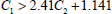
At first glance, any monotonic decreasing function to assign cost to warning cells based on its distance d_min to the closest occupied cell, would seem to work. However this is not the case. For example, Fig. 5 shows two alternative paths T₁ and T₂ that are safer than path T₃. Let V_Ti be the cost associated to path T_i. The robot will prefer path T₁ to path T₃ if V_T3 > V_T1. If the distance between adjacent cells are 1 and $\sqrt{2}$ (for the diagonal), C₁ and C₂ denote costs of warning cells, and we use equation (4) with C_g(i, j)=0, then

$$(C_1+1)\sqrt{2}+(C_1+1)>(C_2+1)+(C_2+1)\sqrt{2}+(C_1+1)\sqrt{2}$$

and hence

$$C_1>2.41C_2+1.141$$

(6)

Fig. 5.

Possible paths to go from R to G. T₁ and T₂ are safer than T₃.

In the case of path T₂, the condition is

$$C_1>6.24C_2+2.84$$

(7)

To minimize the risk of collisions, restrictions given by equations 6 or 7 (for a more conservative and safer path) should be considered in the function C for warning cells, at least for the cells near to obstacles.

2.3.2. Efficiency considerations

To reduce the time to compute an exploration policy, two strategies are considered: (i) Instead of including all unexplored cells as goals, we only include the unexplored cell (or cells) nearest to the robot, and (ii) During the updating process of the value iteration algorithm we use a bounding box (Thrun, S., 1998b). The idea is to update only cells inside a rectangle or box.

2.4. Step 5: Position Tracking

We apply a Markov localization framework (Fox, D. & Burgard, W., 1998) to estimate the most probable location for the robot. The key idea of Markov localization is to compute a probability distribution over all possible locations in the environment. Let P(L_t = l) denote the probability of finding the robot at location l at time t. Here, l is a location in x-y-θ_i space where x and y are Cartesian coordinates of cells, and θ_i is a valid orientation. P(L_t) is updated whenever:

1. The robot moves

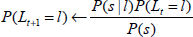
Robot motion is modeled by a conditional probability, denoted by P_a(l | l′). Pa (l | l′) denotes the probability that motion action a, when executed at l′, carries the robot to l. P_a (l | l′) is used to update the belief upon robot motion:

$$P(L_{t+1}=l)\leftarrow \frac{\sum _{l^{\mathrm{\prime }}}{P}_a(l\mid l^{\mathrm{\prime }})P(L_t=l^{\mathrm{\prime }})}{P(s)}$$

(8)

Here P(s) is a normalizer that ensures that P(L_t+1) sums up to 1 over all l. Figure 6 shows an example of Pa(l | l′), considering that the orientation of the robot is aligned to one of the 8 possible directions θ_i, as it was described in a previous section. High probability values are assigned to the transitions from one cell to adjacent cells and low values to the other two cases.

Fig. 6.

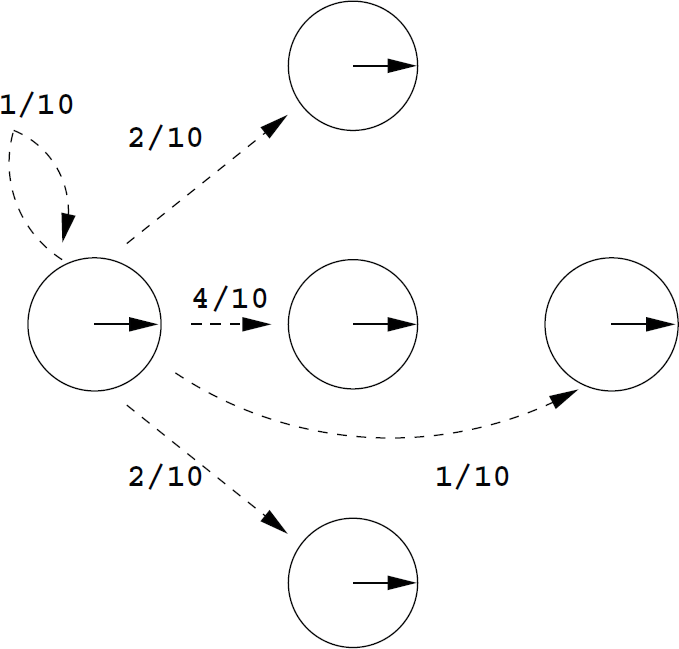
Robot motion for one direction.

2. The robot senses

When sensing s,

$$P(L_{t+1}=l)\leftarrow \frac{P(s\mid l)P(L_t=l)}{P(s)}$$

(9)

Here P(s | l) is the probability of perceiving s at location l. To compute P(s | l) we apply polar correlations between a sensor view (a view built using data from actual sensors) and map views (views computed from the map and all possible locations l). The outcome of the correlation associated to the most probable location is used to align the robot to a valid orientation θ_i.

In order to get an efficient procedure to update the probability distribution, cells with probability below some threshold are set to zero.

Once we know the most probable location l of the robot, we use it in step 2 to fuse sensor data with the map under construction. In our experiments, the robot usually moves through five cells before it gets data from its sensors.

We have described our method to explore and learn a map of an environment, considering a mobile robot with sensors' perceptual limitations. There are several features of the approach that make it a robust exploration method and a better position tracker. In particular: it (i) avoids the risk of collisions with obstacles, (ii) avoids unnecessary rotations (reducing odometric errors), and (iii) minimizes the risk of getting lost when it is far away from obstacles (and hence its sensors are beyond its perceptual limitations).

3. Navigation

Once the map is complete, the same algorithm used for exploration can be used for navigation. In this case, the goal cell takes the place of the unique unexplored cell (a zero value for variable V). In contrast to the exploration phase, during navigation there is no update of the PGM or the travel space.

A significant reduction in the number of free cells to be updated in the value iteration algorithm can be achieved using the travel space associated with the built map. The key idea is to consider travel cells as a kind of road map (as defined in (Latombe, J-C., 1991), a net of roads that the robot will use most of the time to go from one place to another. Some issues must be solved in order to build the road map and use it for navigation. First, how to find the cells of the road map when there are no travel cells in the travel space, e.g., in narrow passages there are only warning cells and the environment can have isolated sets of connected travel cells (see Fig. 7 (a)). Second, how to consider the uncertainty in the position of the robot during navigation. Finally, how to handle cases where the initial and goal position are not within the road map. The following method solves the first problem.

Fig. 7.

Building a roadmap. From left to right: (a) Travel space. (b) Partial roadmap. (c) Full roadmap

Given the distance D_t (the distance between a travel cell and its closest occupied cell) and a cell G of the road map (i.e., a travel cell), we can apply the value iteration algorithm to get a policy of movements to reach cell G. Using this policy, from each warning and travel cell there is a path of cells to the cell G. All the cells of these paths except the first cells (considering the length D_t) form the road map. Fig. 7 (b) shows the road map for the travel space of Fig. 6 (a) using this method. This is a partial road map because there are cells missing for each loop of the full road map. Considering as the goal cell G each of the end cells of the partial road map, a full road map can be built adding the partial road maps (see Fig. 7 (c)). A cell is in the full road map if it is in one or more partial road maps.

The second problem can be solved if the cells in the road map grow in a similar form to the occupied cells in the travel space. In this case, the robot radius is the maximum uncertainty of the robot position.

The last problem can be handled if for each free cell that is not in the road map, it is computed the distance d_min to the nearest cell in the road map (this can be estimated using again the value iteration algorithm without costs for direction changes and type of cells, considering the cells in the road map as the unexplored cells). For a given cell, the cells in a circle of radius d_min connect the given cell to the road map. This approach also solves efficiently the case of very close initial and final positions.

The key idea of this navigation approach is to built a road map from the built map. The road map is a net of safe roads for the robot, like a highway for a car. Because the road map is based on the travel space, and the travel space is built considering the perceptual limitations of sensors, the roads in the road map are easy and safe to follow.

The exploration and navigation are based in the same value iteration algorithm, however when the robot navigates the travel space is fixed. Considering that the number of cells in the road map is a small subset of the free cells, in the future we plan to use the road map idea to solve efficiently the global localization problem.

4. Experimental results

This section presents experimental results obtained using a mobile robot simulator and a real mobile robot.

We consider a differential drive mobile robot. The differential scheme consists of two wheels on a common axis, each wheel driven independently, and two caster wheels to ensure balance. The robot has the ability to drive straight and to turn in place. Our mobile robot, shown in Fig. 8, has an odometer, ultrasonic sensors and a laser range sensor (implemented with a laser line generator and two cameras). The mobile robot base has a micro-controller MC68HC12 to control 2 sonars and 3 DC motors, two for the traction wheels and one to rotate the turret (the top part of the robot). It has a notebook computer (pentium III 1Ghz running Linux Redhat 9) with a wireless network card and a serial connection with the micro-controller.

Fig. 8.

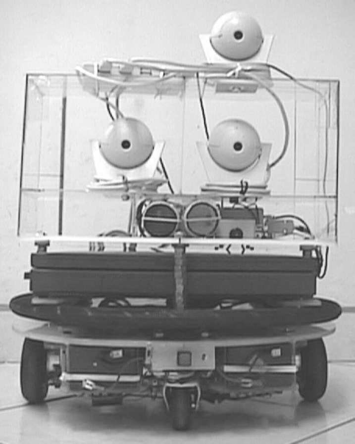
Mobile Robot.

The mobile robot simulator introduces an uniform random error of +/- 3% on rotations and +/- 10% on displacements. When the robot moves forward, the path followed by the robot is not necessarily in the desired direction. The simulator introduces a uniform random variation of +/- 5°.

We consider a PGM with grid cells of 10×10cm² and cells in the travel space with a cost that depends on their type. Far cells have a cost of 600 and travel cells have a cost of 1. Fig. 9 shows the cost of warning cells based on their distance to the nearest obstacles (up to 100 cm). This assignment for the warning cells builds a high repulsive force when the robot is very close to obstacles, 30cm or less, according to Equation 6. Warning cells form a layer of 100 cm and travel cells form a layer of 10 cm.

Fig. 9.

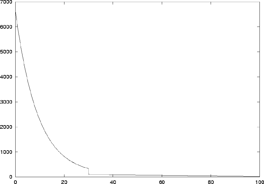
Cost of warning cells depends on the distance (in cm) to the nearest occupied cell.

4.1. Exploration results

Here we present some exploration results using only the travel space. Section 4.2 considers the effect of punishing robot rotations.

First, we considered experiments to observe the effect of using the travel space. Fig. 10 (a) shows a PGM (of about 10×10m²) built by the simulated robot without using the travel space (i.e., assigning null costs to warning and travel cells). The lighter trace on the map is given by the odometer and it shows the path followed by the robot. Note that sometimes the robot gets very close to obstacles.

Fig. 10.

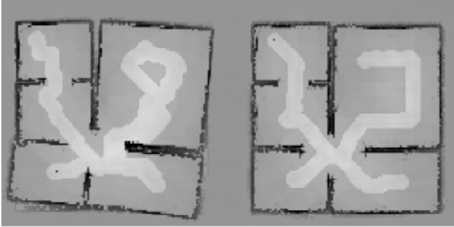
PGMs using the mobile robot simulator. White areas represent cells with occupancy probabilities near to 0. From left to right: (a) Without the travel space. (b) Using the the travel space.

In contrast, Figure 10 (b) shows the map built using the travel space. The costs associated to cells in the travel space implement a kind of wall following strategy to explore the environment, as can be observed in the map. Also the robot does not get too close to obstacles even in narrow passages. Instead, in narrow passages (where there are only warning cells) the robot tends to maximize the clearance between the robot and the obstacles.

The map of the Fig. 10 (b) is also more accurate because the travel space approach tends to move the robot to positions where the sensor readings are more reliable and hence the position tracking algorithm gives better estimations.

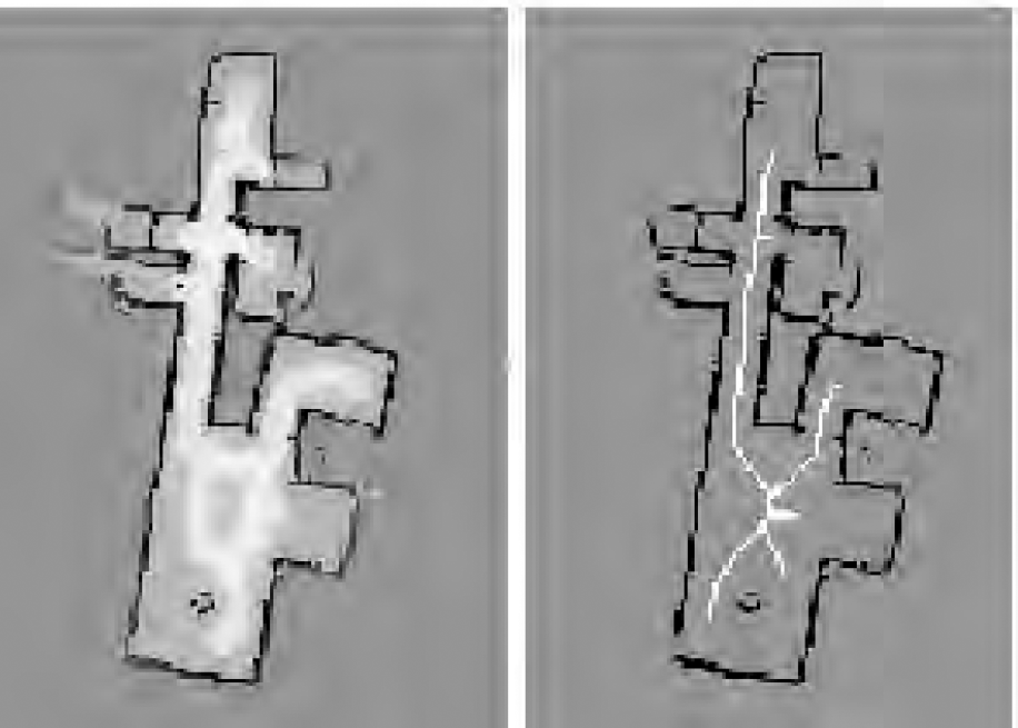
Our next experiments consider the process to build roadmaps. The travel space associated to the map of Fig. 10 (b) is shown in Fig. 11 (a). Travel cells have the lowest cost and they are represented as white pixels. Darker pixels represent free cells with higher costs. For this map, the full set of free cells where the robot can move is shown in Fig. 11 (b). Fig. 11 (c) shows the roadmap extracted from the travel space, using the ideas described before. There is a significant reduction from 6386 free cells (see Fig. 11 (b)), to only 371 cells in the roadmap.

Fig. 11.

From left to right: (a) Travel space associated to map of Fig. 9 (b). (b) Free cells extracted from (a). (c) Roadmap build upon the travel space shown in (a).

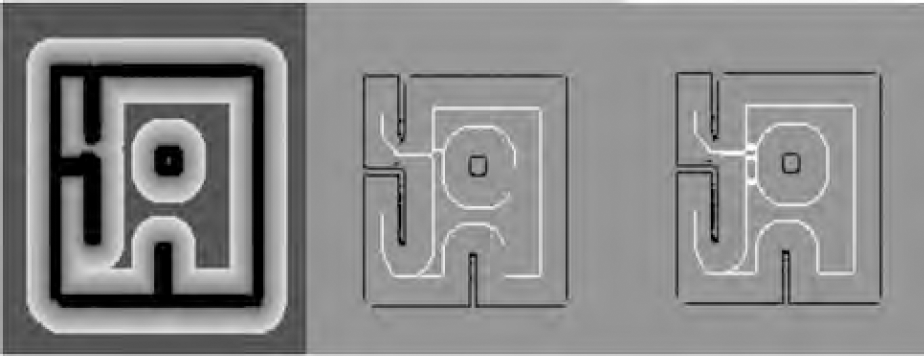
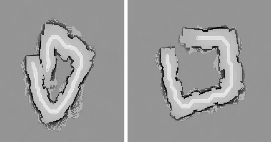
We also test our exploration approach using the real mobile robot. Fig. 12 (a) shows a map of a small house of 8×13m. The built map is accurate enough to be useful for navigation. There are two glass doors in the upper part of the environment that are captured in the map. These are detected by sonars but the laser range finder can see obstacles through them. The road map associated to the built map is shown in Fig. 12 (b).

Fig. 12.

Using the real robot. From left to right: (a) PGM. (b) Roadmap.

Finally we give an example of the three steps of the navigation process. Fig. 13 (a) shows the road map (simulated case) built with an uncertainty on the robot position of 20 cm. Fig. 13 (b) shows two circles that connect the initial and goal cells to the road map (left and right circles respectively) and Fig. 13 (c) shows the motion policy to reach the goal cell given by the value iteration algorithm. In the Fig. 13 (c) darker pixels denote higher values of V that represent higher accumulated costs to reach the goal cell. Note that the goal cell has a cost of zero and it is represented by a white pixel. From these V values, a motion policy for each grid cell is computed using Equation 5.

Fig. 13.

Using the roadmap for navigation. From left to right: (a) Roadmap with an uncertainty of 20 cm. in the position of the robot. (b) The cells of the roadmap and the cells that connect the initial and final cells. (c) Values of V given by the value iteration algorithm (dark pixels denote high values).

4.2. Punishing rotations

The idea of these experiments was to build maps of a simulated environment and compare the total distance, d_T, traveled by the robot wheels, including rotations, for different costs of making rotations of the robot.

If d_T is the distance traveled when the robot moves forward and d_R is the distance traveled when the robot rotates, then the total distance is given by d_T =d_L + d_R. For a differential drive robot with distance D_r (the distance from a traction wheel to the center of the robot), d_R is given by d_R =πD_rg_u /8, where g_u is the rotation of the robot (in units of 45°).

In these experiments we use a linear function to compute C_g (the cost of making rotations of the robot), given by C_g= K_g, where K_g is a constant and g is the rotation (in units of 45°) required by the robot to move to an adjacent cell.

Fig. 14 shows a simulated environment of 12×9m used for these tests. We build 10 maps for this simulated environment with K_g =0 and with K_g=300. These results show that higher K_g values decrease the number of movements that change the orientation of the robot (d_R), and hence the total distance (d_T).

Fig. 14.

Paths followed by the robot. (top) (a) K_g = 0. (bottom) (b) K_g =300.

Statistical information about the time to compute policies of movements (one computation after each movement of the robot) when K_g=0 and K_g =300 show an increment of about 5.3. times when K_g change from 0 to 300. When K_g=0 the algorithm only uses one V variable per cell and when K_g > 0, the algorithm uses the 8 values of V per cell.

Figure 15 shows the PGMs built by the simulated robot without using the position tracking procedure for K_g = 0 and K_g = 300. The grid cells are 10×10 cm². The lighter trace on the map is given by the odometer and it shows the path followed by the robot. Note that the map is worse when K_g =0 (the odometric error is higher).

Fig. 15.

Maps built without using odometric corrections. Dark areas represent cells with occupancy probabilities near to 1. (left) (a) K_g =0. (right) (b) K_g =300

There is a trade of between computation time and movements of the robot. There are fewer rotations and better maps, when rotations are punished (K_g>0) in the value iteration algorithm.

5. Conclusions

A new approach for a mobile robot to explore and navigate in an indoor environment that combines local control (via costs associated to cells in the travel space) with a global exploration and navigation strategy (using a dynamic programming technique) has been described. The new features of our approach are to take explicit account of the actual direction of the robot, reducing odometric errors and building better maps; and an efficient and simple computation of safe paths, based on the cost of cells in the travel space. The paths for the robot are safe because the perceptual limitation of sensors are taken into account in the travel space, so when the robot explores the environment better maps are built.

Previous works do not consider the actual direction of the robot, do not include the computation of safe paths, or are suitable only for exploration (Thrun, S., 1998b; Roy, N., Burgard, W. & Thrun, S., 1998)

As the experimental results confirm, the exploration follows a kind of wall following technique to reduce uncertainty in terms of localization due to sensors' perceptual limitations, as well as to guide the robot through narrow passages, maximizing the distance between the robot and the obstacles. This combination of local and global strategies takes the advantages of both: robustness of local strategies and completeness of global strategies.

In addition, this approach minimizes the number of orientation changes, reducing odometric errors. Experimental results confirm that Kg (the cost associated to rotations) is analog to the effect of an inertial mass: it tends to keep the orientation of the robot unchanged, reducing the total distance traveled by the robot and building more accurate maps. The increment of computation time to compute a policy is about 5.3 times the amount used without punishing rotations. However, with the reduction in the number of cells included in the algorithm and using the bounding box technique, the computation time is small enough to be included within the whole map building process.

A preprocessing of the travel space that results in a road map is used for navigation purposes. It significantly reduces the number of cells to be updated in the value iteration algorithm, and consequently reduces the time to compute the motion policy for the robot. The road map is a net of safe roads that the mobile robot can use for navigation.

In the future, we plan to use this approach to build maps of environments with long cycles. If odometric errors are lower, the position tracking task should be easier. Also we plan to use the road map to solve the global localization problem in an efficient way.