Sage Journals: Discover world-class research

Abstract

This paper presents a problem of fault detection and isolation (FDI) in mechatronic systems described by nonlinear dynamic models with such types of no differentiable nonlinearities as saturation, Coulomb friction, backlash, and hysteresis. To solve this problem, so-called logic-dynamic approach is suggested. This approach consists of three main steps: replacing the initial nonlinear system by certain linear logic-dynamic system, obtaining the bank of linear logic-dynamic observers, and transforming these observes into the nonlinear ones. Logic-dynamic approach allows one to use the linear FDI methods for diagnosis in nonlinear mechatronic systems.

Keywords

mechatronic systems nonlinear models fault detection and isolation observers robustness

1. Introduction and Problem Statements

The problem of fault detection and isolation (FDI) was extensively investigated for the past 20 years; see, e.g., the surveys (Frank, M., 1990; Gertler, J., 1993; Patton, R., 1994; Isermann, R. & Balle, P., 1996), the books (Patton, R. & Frank, P., 2000; Chiang, L. et al, 2001; Blanke, M. et al, 2003). Many problems have been studied and solved: different methods of residual generation and relationships among them, robustness, adaptive threshold test, H∞ approach, fuzzy logic, descriptor systems, different classes of nonlinear systems, inequality constraints, geometric approach and so on. Many practical examples were considered; in particular, special book was devoted to mechatronic systems (Caccavale, F. & Villiani, L., 2002).

The main purpose of this paper is to consider the FDI problem for wide class of mechatronic systems. As a rule, these systems are nonlinear essentially with such types of no differentiable nonlinearities as saturation, Coulomb friction, backlash, and hysteresis. Therefore one has to use nonlinear methods of the FDI. However, most of papers dealing with the FDI problem consider the nonlinear systems with differential nonlinearities (Seliger, R. & Frank, P., 1991; Shields, D., 1996; Staroswiecki, M. & Comtet-Varga, M., 1999; De Persis, C. & Isidori, A., 2001) therefore they cannot be used in our case.

There are several papers developed the algebraic approach to the FDI problem and intended for systems with no differentiable nonlinearities (Zhirabok, A. & Shumsky A., 1987; Zhirabok, A. & Preobrazhenskaya, O., 1994; Zhirabok, A., 1997). However, they require rather complex analytical transformations therefore it is difficult to use them in practice. This paper is intended to overcome these difficulties and develop an approach allowing one to solve the FDI problem for a wide class of mechatronic systems. So-called logic-dynamic approach is suggested to obtain the simple FDI procedure in systems with no differentiable nonlinearities.

This paper is a logical sequel of (Filaretov, V. et al 1999, 2003) where the FDI problem in robots in operation was studied. The FDI process in (Filaretov, V. et al 1999) was provided by the bank of observers. It was shown that the observer-based approach does not allow one to distinguish some faults even though all elements of the state vector are measured. To overcome this difficulty, the parity space approach was used in (Filaretov, V. et al 2003), which allowed one to distinguish these faults. It is well-known (Gertler, J., 1993) that in the linear case the observer-based approach and the parity space one are equivalent. It was shown in (Filaretov, V. et al 2003) that there are nonlinear systems for which the parity equations cannot be obtained. At the same time, the observer-based approach can be used in this case. Therefore, in the nonlinear case, these approaches are not equivalent and must be used in combination for fault diagnosis in complex technical systems.

The paper is organized as follows. Section 2 describes the main models under consideration. Section 3 is devoted to the logic-dynamic approach. Firstly, the main steps of this approach are given. Then the first and second steps are described in detail. In Section 4, four conditions of the observer existence are obtained. Section 5 is devoted to the observer design, and the third step of the suggested approach is described. In Section 6, the problem of stability is discussed. Modifications of the logic-dynamic approach are suggested in Section 7. An example is considered in Section 8. Section 9 concludes the paper.

2. Basic Models

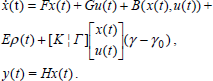
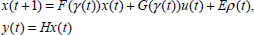
In this paper, the logic-dynamic approach is developed for a class of nonlinear systems described by the equations

\begin{aligned} \dot{x} (t) = F (γ (t)) x (t) + G (γ (t)) u (t) + B (x (t), u (t)) + E ρ (t), \\ y (t) = H x (t) . \end{aligned}

Here x, y, and u are the vectors of state, output, and control; γ is the function presenting the faults; F(γ), G(γ), and B(x,u) are matrix functions; H and E are known matrices of appropriate dimensions. The term Eρ(t) models unknown parameters and unknown inputs to the actuator and to the dynamic process; the evaluation of the vector function ρ(t) must generally be considered unknown. It is supposed also that if there are no faults, then γ(t) = γ₀; if a fault occurs, γ(t) becomes an unknown function. Notice that the case when the function B(x,u) has the form B(y,u) was considered in (Frank, P., 1990).

Write down the approximate equalities

\begin{aligned} F (γ) = F (γ_{0}) + \frac{d F}{d γ} |_{γ = γ_{0}} (γ - γ_{0}) = F + K (γ - γ_{0}), \\ G (γ) = G (γ_{0}) + \frac{d G}{d γ} |_{γ = γ_{0}} (γ - γ_{0}) = G + Γ (γ - γ_{0}), \end{aligned}

and substitute the last expressions for the matrices F(γ(t)) and G(γ(t)):

\begin{aligned} \dot{x} (t) = F x (t) + G u (t) + B (x (t), u (t)) + \\ E ρ (t) + [K \begin{matrix} \binom{|}{|} \end{matrix} Γ] [\begin{matrix} x (t) \\ u (t) \end{matrix}] (γ - γ_{0}), \\ y (t) = H x (t) . \end{aligned}

(1)

Denote system (1) with F = F(γy₀) and G = G(γ₀) as ∑ = (F,B,G,H)

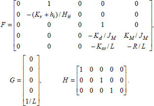
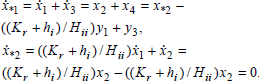
As a practical example, consider the general electric servoactuator of manipulation robots studied in (Filaretov, V. et al 1999, 2003). The servoactuator dynamic, with the backlash and elasticity taken into account, may be described by the following nonlinear equations:

\begin{aligned} {\dot{x}}_{1} = x_{2}, \\ {\dot{x}}_{2} = (1 / H_{i i}) (- (K_{r} + h_{i}) x_{2} - M_{r} + C_{r} i_{r} B l (x_{3} - i_{r} x_{1})), \\ {\dot{x}}_{3} = x_{4}, \\ {\dot{x}}_{4} = (1 / J_{M}) (- K_{d} x_{4} + K_{M} x_{5} - M_{d} - C_{r} B l (x_{3} - i_{r} x_{1})), \\ {\dot{x}}_{5} = (1 / L) (- K_{ω} x_{4} - R x_{5} + u) . \end{aligned}

Here x₁ and x₂ are the output rotation angle and velocity at the reducer output shaft, respectively; x₃ and x₄ are the output rotation angle and velocity at the motor output shaft, respectively; x₅ is the current through the servoactuator windings; H_ii and h_i are the components of the inertia and velocity, respectively: M_d and M_r are the moments of the Coulomb friction at the motor and reducer shaft output, respectively: M_d = M_dosign(x₄), M_r = M_rosign(x₂); K_d and K_r are the respective coefficient of viscous friction of the motor and reducer output shaft; i_r is the reducing ratio of the reducer; C_r is the rigidity coefficient of the mechanical reducer; J_M is the moment of inertia of the electric servoactuator and of the rotating parts of the reducer; K_ω and K_M 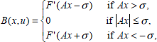are the respective coefficients of the counter EMF and of the torque; R and L are the active and inductive resistances of the electric servoactuator windings, respectively; the function Bl describes the backlash:

B l (z) = 0.5 (| z | - σ) (s i g n (z + σ) + s i g n (z - σ)),

2σ is the backlash span, $z = x_{3} - i_{r} x_{1}$ .

3. Logic-dynamic Approach

The logic-dynamic approach to solve the FDI problem for system (1) includes the following steps (Zhirabok, A. & Usoltsev S., 2002).

Replacing the initial nonlinear system (1) by so-called linear logic-dynamic (LLD) system containing several linear subsystems and linear logical conditions.

Solving the FDI problem for the LLD system and obtaining the bank of the LLD observers.

Transforming the LLD observers into the nonlinear ones.

For detail description of the logic-dynamic approach, consider the simple case with single nonlinearly (Coulomb friction) of the form

B (x (t), u (t)) = G^{'} u (t) s i g n (A x (t))

(2)

for certain matrix G′ and row matrix A.

On the first step of this approach, replace the system ∑ = (F,B,G,H), by certain LLD system. This system consists of three linear subsystems

\begin{aligned} Σ_{1} = (F, B, G - G^{'}, H), \\ Σ_{2} = (F, 0, G, G), \\ Σ_{3} = (F, 0, G + G^{'}, H), \end{aligned}

with two linear logical conditions Ax(t) ≥ 0 and Ax(t) > 0 (see Fig. 1). If the condition Ax(t)<0 holds, then (in the unfaulty case with ρ(t) = 0) model (1) reduces to ∑₁:

\dot{x} (t) = F x (t) + (G - G^{'}) u (t),

if Ax(t) = 0, then to ∑₂:

\dot{x} (t) = F x (t) + G u (t),

if Ax(t) > 0, then to ∑₃:

\dot{x} (t) = F x (t) + (G + G^{'}) u (t);

y(t) = Hx(t) for the systems ∑₁ – ∑₃. It is very important that these models have the identical matrices F and H.

Fig. 1.

Structure of logic-dynamic system

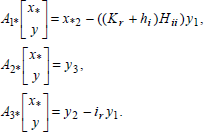
On the second step, a bank of the LLD observers has to be obtained. Assume that a structure of the LLD observer is similar to the one shown in Fig. 1, therefore three subsystems ∑_*1,∑_*2,∑_*3 and the row matrix A_* exist such that the following relationships hold:

if A_*x_*(t) < 0, then the LLD observer reduces to ∑_*1:

{\dot{x}}_{*} (t) = F_{*} x_{*} (t) + (G_{*} - G_{*}^{'}) u (t) + J_{*} y (t),

if A_*x_*(t) = 0, then ∑_*2:

{\dot{x}}_{*} (t) = F_{*} x_{*} (t) + G_{*} u (t) + J_{*} y (t),

(3)

if A_*x_*(t) > 0 then ∑_*3:

{\dot{x}}_{*} (t) = F_{*} x_{*} (t) + (G_{*} + G_{*}^{'}) u (t) + J_{*} y (t);

y_*(t) = H_*x_*(t) for the systems ∑_*1 – ∑_*3. Here x_*(t) is the state vector of the observer, y_*(t) is the output vector, F_*, G_*, J_*, and H_* are constant matrices; it is assumed that the matrix F_* is stable. The observer generates the residual

r (t) = C y (t) - y_{*} (t)

for certain matrix C which has to be determined. If there are no faults and ρ(t) = 0, then r(t) = 0, if a fault occurs, r(t) ≠ 0.

It is well-known from the linear FDI theory (Frank, P., 1990; Gertler, J., 1993; Patton R., 1994; Zhirabok, A., 1997) that for the observer design, the matrix Φ such that

Φ x (t) = x_{*} (t)

in the unfaulty case after the response to unlike conditions have died out plays the main role. In the absence of faults, the following well-known set of equations holds (Frank, P., 1990; Patton R., 1994; Zhirabok, A., 1997):

H_{*} Φ = C H, Φ F = F_{*} Φ + J_{*} H, G_{*} - Φ G .

(4)

To ensure the reliable fault detection, the residual r(t) has to be sensitive to the faults and invariant with respect to the unknown inputs ρ(t) that is

Φ [K \begin{matrix} \binom{|}{|} \end{matrix} Γ] \neq 0, Φ E = 0 .

(5)

To fit the logical conditions in the initial LLD system to the ones in the LLD observer, assume that the following relationships hold in the unfaulty case:

\begin{aligned} if A x (t) < 0, then A_{*} x_{*} (t) < 0, \\ if A x (t) = 0, then A_{*} x_{*} (t) = 0, \\ if \forall x (t) > 0, then A_{*} x_{*} (t) > 0 . \end{aligned}

Since x_*(t)=Φx(t), i.e. A_*x_*(t)=AΦx(t), then these relationships hold if $A = A_{*} Φ$ . Because of this, each row of the matrix A is a linear combination of the matrix Φ rows therefore this equality is equivalent to the rank condition

rank (Φ) = rank [\begin{matrix} Φ \\ A \end{matrix}] .

(6)

This condition imposes an additional restriction on the matrix Φ.

4. Observer Existence Conditions

4.1. Preliminary rezults

To design an observer in the linear case, there are a number of approaches, e.g., the eigenstructure assignment (Patton R., 1994), the approach based on the Kronecker canonical form (Frank, P., 1990). Consider another linear procedure suggested in (Mironovsky, L., 1979; Zhirabok, A., 1997) also based on the Kronecker canonical form that allows one to take into account condition (6) easily.

It is well-known (Kwakernaak, H. & Sivan, R., 1972) that the matrices F_* and H_* describing the observer can be represented in a canonical form with the matrices

F_{*} = [\begin{matrix} β_{1} & 1 & 0 & \dots & 0 \\ β_{2} & 0 & 1 & \dots & 0 \\ . & . & . \\ β_{k} & 0 & 0 & \dots & 0 \end{matrix}], H_{*} = [1 0 0 \dots 0]

without increasing their dimensions. By analogy with (Mironovsky, L., 1979; Zhirabok, A., 1997), transform the observer with these matrices into the open-loop observer with the matrices

F_{*} = [\begin{matrix} 0 & 1 & 0 & \dots & 0 \\ 0 & 0 & 1 & \dots & 0 \\ . & . & . \\ 0 & 0 & 0 & \dots & 0 \end{matrix}], H_{*} = [1 0 0 \dots 0] .

(7)

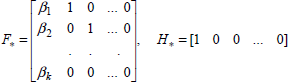
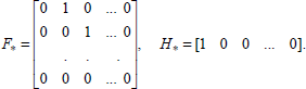
This can be arranged by removing the feedback coefficients β₁, β₂, …, β_k and transforming the matrix J_*. This transformation allows one to obtain a simple algorithm of the observer design.

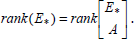
Let E_* be a matrix of maximal rank satisfying the equality E_*E = 0 . It follows from this definition that expression ΦE = 0 can be rewritten as Φ = NE_* for some matrix N.

There are several conditions of existence the observer invariant with respect to ρ(t).

4.2. The first condition

Consider the first equation in (4) $H_{*} Φ = C H$ ; due to the equality $Φ = N E_{*}$ and (7), it can be written in the form $N_{1} E_{*} = C H$ or

[N_{1} ∣ - C] \cdot [\begin{matrix} E_{*} \\ H \end{matrix}] = 0

(8)

where N₁ is the first row of the matrix N. Clearly from (8) that rows of the matrices E_* and H are linearly dependent, therefore equation (8) is equivalent to the rank inequality

r a n k [\begin{matrix} E_{*} \\ H \end{matrix}] < r a n k (E_{*}) + r a n k (H)

(9)

under the assumption that the matrix H is of full rank. If it is true, the matrices C⁰ and

N_{1}^{0}

of maximal rank can be obtained from equation (8); the rows of these matrices are all linear independent solutions of (8). The matrices C and N₁ can be obtained from the matrices C⁰ and

N_{1}^{0}

as follows:

C = Q C^{0}, N_{1} = Q N_{1}^{0}

for certain matrix Q which has to be determined.

If condition (9) does not hold, the observer invariant with respect to ρ(t) cannot be built.

4.3. The second condition

Consider the second equation in (4) $F_{α} Φ + J H = Φ F$ . Multiply it by E and take into account the equalities $Φ = N E_{*}$ and ΦE = 0 that gives, by analogy with (8), the equation

[N ∣ - J] \cdot [\begin{matrix} E_{*} F E \\ H E \end{matrix}] = 0 .

(10)

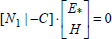
As above, this equation is equivalent to the rank condition

rank [\begin{matrix} E_{*} F E \\ H E \end{matrix}] < rank (E_{*} F E) + rank (H E)

(11)

under the assumption that the matrices E_*FE and HE are of full rank. If it is true, the matrices N and J exist such that equation (10) holds; rewrite it in the form

(N E_{*} F - J H) E = 0 .

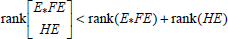
It follows from definition of the matrix E_* that the last equation is equivalent to the equation

N E_{*} F - J H = K E_{*}

(12)

for some matrix K. Take

N E_{*} = Φ

and K = F_*N for some matrix F_*, then

K E_{*} = F_{*} N E_{*} = F_{*} Φ

and equation (12) coincides with the second equation in (4). This can be taken into account as follows. The matrices N⁰ and J⁰ of maximal rank can be obtained from equation (10); rows of these matrices are all linear independent solutions of (10). These matrices can be used as the basis for the observer design; minimal dimension of this observer and the matrices N and J have to be determined in this case that is not a trivial task. Another way to observer design based on the canonical form of the matrix F_* from (7) to simplify a design procedure will be suggested.

If condition (10) does not hold, the observer invariant with respect to ρ(t) cannot be built.

4.4. The third condition

Consider the matrices $N_{1}^{0}$ and N⁰ obtained from equations (8) and (10), respectively. Because these equations are independent one another, these matrices are also independent. Because rows of the matrix N are linear combinations of the matrix N⁰ rows and $N_{1} = Q N_{1}^{0}$ , then $N_{1} = Q N_{1}^{0} = W N^{0}$ for some matrix W or, by analogy with the first condition,

r a n k [\begin{matrix} N_{1}^{0} \\ N^{0} \end{matrix}] < r a n k (N_{1}^{0}) + r a n k (N^{0}) .

(13)

This inequality may be named as concordance condition of equations (8) and (10). If condition (13) does not hold, the observer cannot be built.

4.5. The fourth condition

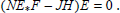
The last condition follows from nonlinear feature of system (1). As it shown above, $A = A_{*} Φ$ ; because $Φ = N E_{*}$ , then $A = A_{*} N E_{*}$ or, in the rank form,

r a n k (E_{*}) = r a n k [\begin{matrix} E_{*} \\ A \end{matrix}] .

(14)

If this condition does not hold, a nonlinear observer corresponding to the system in the form (1) and invariant with respect to ρ(t) cannot be built.

5. Observer Design

5.1. Preliminary results

If one of conditions (9), (11), and (14) does not hold, the observer invariant with respect to ρ(t) cannot be built. In this case one has to use the robust methods, which allows one to minimize the influence of ρ(t) on r(t) (see Low, X. at al, 1984; Frank, P., 1990).

Assume that conditions (9), (11), (13), and (14) hold. Using matrices in (7), one can obtain from (4) with C = QC⁰ the following equations:

\begin{aligned} Φ_{1} = Q C^{0} H, Φ_{i} F = Φ_{i + 1} + J_{* i} H, \\ i = 1, 2, \dots, k - 1, J_{* k} H = Φ_{k} F, \end{aligned}

(15)

where Φ_i and J_*i are the i-th rows of the matrices Φ and J_*, respectively.

Consider the second equation in (15) with i=1 and replace the matrix Φ₁ by RC⁰H:

Q C^{0} H F = J_{* 1} H F + Φ_{2} .

Multiple this equation by F and replace the product Φ₂F by $J *_{2} H + Φ_{3}$ according to the second equation in (15) with i=2:

Q C^{0} H F^{2} = J_{* 1} H F + J_{* 2} H + Φ_{3} .

Eventually one can obtain the single equation

Q C^{0} H F^{k} = J_{* 1} H F^{k - 1} + J_{* 2} H F^{k - 2} + \dots + J_{* k} H .

(16)

This equation is a basis of the suggested algorithm to design the observer, i.e. to find the matrices Q, J_*1, J_*2,…, J_*k, G_*, G_*, and A_*.

5.2. Algorithm

Step 1.
Let k=1.
Step 2.
If equation (16) holds for some row matrices Q, J_1, J_2,…, J_k (this can be checked using the mathematical packages, e.g. MATLAB), go to 4.
Step 3.
Let k=k+1; if k≤n, go to 2, otherwise the observer satisfying condition (5) and (6) cannot be built.
Step 4.
Obtain the rows of the matrix $Φ : Φ_{1} = Q C^{0} H, Φ_{i + 1} = Φ_{i} F - J_{ i} H, i = 1, 2, \dots, k - 1$ . If the matrix Φ does not satisfy conditions (5) or (6), find another solution of equation (16) otherwise go to 3.
Step 5.
Let $G_{}^{'} = Φ G^{'}, G_{} = Φ G, C = Q C^{0}$ and obtain the row matrix A_* from the linear algebraic equation $Φ A_{*}^{T} = A^{T}$ End.

Notice that the matrix Q can be specified in some cases.
5.3. Nonlinear observer design

On the third step of the suggested approach, it is necessary to transform the obtained LLD observer into the nonlinear one. Recall that to obtain the LLD system, the initial nonlinear system is replaced by three linear subsystems ∑₁, ∑₂, ∑₃ and two logical conditions Ax(t) ≥ 0 and Ax(t) < 0 obtained by removing the nonlinear term

B (x (t), u (t)) = G^{'} u (t) s i g n (A x (t))

from (1). In its turn the LLD observer is represented by three linear subsystems ∑_*1, ∑_*2, ∑_*3 and two logical conditions

A_{*} x_{*} (t) \geq 0

and

A_{*} x_{*} (t) < 0

Therefore to obtain the nonlinear observer, one has to perform the inverse process, i.e. the term G_*u(t)sign(A_*x_*(t)) must be added to the right-hand side of equation (3):

{\dot{x}}_{*} (t) = F_{*} x_{*} (t) + G_{*} u (t) + J_{*} y (t) + G_{*}^{'} u (t) s i g n (A_{*} x_{*} (t)) .

(17)

6. Stability of Observer

To obtain a stable matrix F_* in equation (4), it is necessary to use a feedback in the observer and to correct the matrix J_* correspondingly. Namely, if β₁, β₂, …, β_k are the feedback coefficients providing the necessary stability of this matrix, then the i-th row J_*i of the matrix J_* has to be replaced by the row $J *_{i} - β_{i} C, i = 1, 2, \dots, k$ It is very important that the matrix Φ does not change in this case therefore the main properties of the observer (invariance with respect to the function ρ(t) and sensitivity to the faults) are not changed also. Actually, consider the i-th (i <k) row of the second matrix equation in (4), the matrix F_* with the coefficients β₁, β₂, …, β_k and the row matrix J_*i replaced by $J *_{i} - β_{i} C$

β_{i} Φ_{1} + Φ_{i + 1} + (J *_{i} - β_{i} C) H = Φ_{i} F .

Since CH = Φ₁, it is easy to obtain the second term in (15) from this expression; the same is true for i=k. Therefore, the matrix Φ obtained from Algorithm is left unchanged under that change in the matrix F_*. Thus, the problems of the observer invariance with respect to ρ(t) and stability of the matrix F_* can be solved independently of each other.

The transformation of the LLD observer into the nonlinear one can change stability of the observer. In this case, to obtain the asymptotically stable observer, equation (17) describing the observer has to be supplemented by the term $G_{0} (x_{*} (t), u (t), y (t)) r (t)$

\begin{aligned} {\dot{x}}_{*} (t) = F_{*} x_{*} (t) + G_{*} u (t) + J_{*} y (t) + J_{*} y (t) + G_{*}^{'} u (t) s i g n (A_{*} x_{*} (t)) + \\ G_{0} (x_{*} (t), y (t)) r (t) . \end{aligned}

where G₀ is a gain matrix function. The problem of this matrix finding was extensively studied in literature; see, e.g., survey (Misawa, E. & Hedrick, J., 1989), papers (Birk, J. & Zeitz, M., 1988; Ding, X. & Frank, P., 1990). For this reason this problem is not considered in this paper.

7. Modifications of Suggested Approach

7.1. Some extensions

As it follows from the logic-dynamic approach, the matrix G' in (2) can be replaced by the matrix function G' (u, γ) or G (u, y, γ); in this case the additional term in (17) is of the form $Φ G^{'} (u, γ_{0}) s i g n (A_{*} x_{*})$ or $Φ G^{'} (u, y, γ_{0}) s i g n (A_{*} x_{*})$ , respectively.

If there exist several nonlinearities in system (1) with matrices $G_{1}^{'}, G_{2}^{'}, \dots, G_{p}^{'}$ and A₁, A₂, …, A_p, one has to form the compound matrix

A = [A_{1}^{T} A_{2}^{T} \dots A_{p}^{T}]^{T}

and use it as pointed above.

The logical conditions in the LLD observers $A_{*} x_{*} (t) < 0$ or $A_{*} x_{*} (t) = 0$ , or $A_{*} x_{*} (t) > 0$ can be relaxed by extension of the vector x_* with the vector y as follows:

A * [\begin{matrix} x * \\ y \end{matrix}] < 0 or A * [\begin{matrix} x * \\ y \end{matrix}] = 0, or A * [\begin{matrix} x * \\ y \end{matrix}] < 0 .

(18)

In this case, condition (6) must be replaced by the one

rank [\begin{matrix} Φ \\ H \end{matrix}] = rank [\begin{matrix} Φ \\ H \\ A \end{matrix}] .

(19)

Besides, condition (14) is relaxed in this case and is of the form

rank [\begin{matrix} E * \\ H \end{matrix}] = rank [\begin{matrix} E * \\ H \\ A \end{matrix}] .

(20)

However, it becomes necessary condition only for the following reason. Suppose that each row in the matrix A is a linear combination of the matrices E_* and H rows. However, from this it does not follow that they are linear combinations of the matrices Φ = NE_* and H rows. Therefore, if equality (20) holds, condition (19) must be checked. If condition (20) does not hold, the observer invariant with respect to ρ(t) cannot be built.

It is known that for the system described by the difference equations

\begin{aligned} x (t + 1) = F (γ (t)) x (t) + G (γ (t)) u (t) + E ρ (t), \\ y (t) = H x (t) \end{aligned}

and for the observer described in the same manner as (3), relationships (4) and (5) hold. Thus, the logic-dynamic approach can be extended on the discrete-time case.

The suggested approach has been described in Sections 2 and 3 to fit a task of fault detection. It can be easily to transform it for fault isolation. Actually, consider the following form of model (1):

\begin{aligned} \dot{x} (t) = F x (t) + G u (t) + B (x (t), u (t)) + E ρ (t) + \\ \sum_{i = 1}^{q} K_{i} x (t) (γ_{i} (t) - γ_{i 0}) + \sum_{i = 1}^{q} Γ_{i} u (t) (γ_{i} (t) - γ_{i 0}), \\ y (t) = H x (t), \end{aligned}

where the function γ_i (t) describes the i-th fault f_i: if this fault occurs, γ_i(t) becomes an unknown function, otherwise

γ_{i} (t) = γ_{i 0}

; K_i and Γ_i are matrices, i=1,2,…,q. In this case, the bank of observers has to be obtained. For example, if the j-th observer has to be invariant with respect to the faults

f_{j 1}, f_{j 2}, \dots, f_{j v}

then in addition to the condition ΦE=0 in (5), the following equations have to hold:

Φ K_{j 1} = 0, Φ K_{j 2} = 0, \dots, Φ K_{j v} = 0, Φ Γ_{j 1} = 0, Φ Γ_{j 2} = 0, \dots, Φ Γ_{j v} = 0

. They can be combined into the single one:

Φ [E K_{j 1} K_{j 2} \dots K_{j v} Γ_{j 1} Γ_{j 2} \dots Γ_{j v}] = 0 .

A demand of sensitivity to the rest faults yields the set of inequalities:

Φ [K_{i}] \neq 0, Φ [Γ i] \neq 0, i \notin {j_{1}, j_{2}, \dots, j_{v}} .

The numbers $j_{1}, j_{2}, \dots, j_{v}$ are defined from the j-th row of the special matrix of faults D, or coding set (Gertler, J., 1993; Zhirabok, A., 1994). The matrix D reflects sensitivity/insensitivity of the observer to the faults: if the j-th observer is sensitive to the fault f_i, then $D [j, i] = 1$ , otherwise $D [j, i] = 0$ . The algorithm of the matrix D obtaining is suggested in (Zhirabok, A., 1994).

In this case, r(t) is a vector of residuals; decision making has to be performed on the basis of the matrix D. The matrix $[E K_{j 1} K_{j 2} \dots K_{j v} Γ_{j 1} Γ_{j 2} \dots Γ_{j v}]$ has to be used instead of the matrix E to obtain the matrices E_* and C by analogy with Section 4.

7.2. Another types of nonlinearities

Consider another type of nonlinearity – a backlash described by the model $B (x, u) = F^{'} B l (A x - σ)$ , or

B (x, u) = {\begin{cases} F^{'} (A x - σ) & if A x > σ, \\ 0 & if | A x | \leq σ, \\ F^{'} (A x + σ) & if A x < - σ, \end{cases}

where 2σ is the backlash span and F' is a certain matrix. In this case, it is impossible to use directly the approach suggested above because it gives the systems ∑₁, ∑₂, ∑₃ with different dynamics:

\begin{aligned} Σ_{1} = (F + F^{'} A, 0, G, H), \\ Σ_{2} = (F, 0, g, H), \\ Σ_{3} = (F + F^{'} A, 0, G, H) . \end{aligned}

To overcome this difficult, assume that the model of observer contains the term analogous to $B (x, u) = F^{'} B I (A x - σ)$

B * (x *, u) = F_{*}^{'} B I (A * x * - σ *) .

Matrices Φ and A_* are determined from Algorithm therefore the second equation in (4) holds for the system $Σ_{2} : F_{*} Φ + J * H = Φ F$ . Let $F_{*}^{'} = Φ F^{'}$ and $σ_{*} = σ$ , then the second equation in (4) holds for the systems ∑₁ and ∑₃. Actually, since $S * Φ = A$ , then $F_{*}^{'} A * A * Φ = Φ F^{'} A$ therefore

F_{*} Φ + J * H + F_{*}^{'} A * Φ F + Φ F^{'} A,

(F_{*} + F_{*}^{'} A *) Φ + J * H = Φ (F + F^{'} A)

follows from this equality and the equation

F_{*} Φ + J * H = Φ F

Therefore, the task is reduced to that considered in Section 3 with restriction (6).

Two another types of no differentiable nonlinearities (saturation and hysteresis) can be considered by analogy, and they give analogous results. Moreover, the suggested approach can be used for another types of nonlinearities such as G' u(t)sin(Ax), G' u(t)cos(Ax), G' u(t)log(Ax) and so on. Actually, consider the term G' u(t)sign(Ax) and $G_{*}^{'} u (t) s i g n (A * x *)$ in the initial system and the observer, respectively. Clearly, the last term is a result of certain transformation of the first one, and the LLD approach gives a rule of this transformation. Therefore, the nonlinearity G' u(t)sin(Ax) in the initial system gives the term G'_*u(t)sin(A_*x_*) in the observer in spite of the fact that it is impossible to transform system (1) into any LLD system in this case. Here restriction (6) (or (19)) reflects not a logical condition but a condition of concordance of nonlinearities in the initial system and in the observer.

8. Example

Consider the general electric servoactuator of manipulation robots with dynamics described in Section 2. Assume that

y_{1} (t) = x_{1} (t), y_{2} (t), y_{2} (t) = x_{3} (t), y_{3} (t) = x_{4} (t) .

The corresponding LLD system is described by the following matrices:

\begin{aligned} F & = [\begin{matrix} 0 & 1 & 0 & 0 & 0 \\ 0 & - (K_{r} + h_{r}) / H_{i i} & 0 & 0 & 0 \\ 0 & 0 & 0 & 1 & 0 \\ 0 & 0 & 0 & - K_{d} / J_{M} & K_{M} / J_{M} \\ 0 & 0 & 0 & - K_{ω} / L & - R / L \end{matrix}], \\ G = [\begin{matrix} 0 \\ 0 \\ 0 \\ 0 \\ 1 / L \end{matrix}], H = [\begin{matrix} 1 & 0 & 0 & 0 & 0 \\ 0 & 0 & 1 & 0 & 0 \\ 0 & 0 & 0 & 1 & 0 \end{matrix}] . \end{aligned}

Assume that faults and unknown inputs are described as follows:

G = [\begin{matrix} 0 \\ 1 \\ 0 \\ 0 \\ 0 \end{matrix}], E = [\begin{matrix} 0 \\ 0 \\ 0 \\ 1 \\ 0 \end{matrix}], Γ = [\begin{matrix} 0 \\ 0 \\ 0 \\ 0 \\ 0 \end{matrix}] .

Because of several types of nonlinearities, the term B(x,u) in (2) is in the form $B (x, u) = (G^{'} u + D) W (x)$ therefore the corresponding term in the observer is $(G_{*}^{'} + D *) W *$ with $G_{*}^{'} = Φ G^{'}, D * = Φ D$ . Here

\begin{aligned} G^{'} = 0, W (x) = [\begin{matrix} s i g n (A_{1} x) \\ s i g n (A_{2} x) \\ B 1 (A_{3} x) \end{matrix}], \\ D = [\begin{matrix} 0 & 0 & 0 \\ - M_{r o} / H_{i i} & 0 & C i_{r} / H_{i i} \\ 0 & 0 & 0 \\ 0 & - M_{d o} / J_{M} & - C / J_{M} \\ 0 & 0 & 0 \end{matrix}], \\ A_{1} = [0 1 0 0 0], \\ A_{2} = [0 0 0 1 0], \\ A_{3} = [- i_{r} 0 1 0 0] \\ W * (x *) = [\begin{matrix} s i g n (A_{1} * x *) \\ s i g n (A_{2} * x *) \\ B 1 (A_{3} * x *) \end{matrix}] \end{aligned}

if (6) holds and

W * (x *, y) = [\begin{matrix} s i g n (A_{1} * [x_{*}^{T} ∣ y^{T}]^{T}) \\ s i g n (A_{2} * [x_{*} T ∣ y^{T}]^{T}) \\ B 1 (A_{3} * [x_{*}^{T} ∣ y^{T}]^{T}) \end{matrix}]

if (19) holds.

Perform the necessary calculations. It follows from E_*E=0 that

E * = [\begin{matrix} 1 & 0 & 0 & 0 & 0 \\ 0 & 1 & 0 & 0 & 0 \\ 0 & 0 & 1 & 0 & 0 \\ 0 & 0 & 0 & 0 & 1 \end{matrix}] .

Because $rank (E *) = 4, rank (H) = 3$ , and $rank [\begin{matrix} E * \\ H \end{matrix}] = 5$ , then condition (9) holds. One can show that $rank (E * F E) = 1, rank (H E) = 1$ , and $rank [\begin{matrix} E * F E \\ H E \end{matrix}] = 1$ , then condition (11) holds. It follows from (8) and (10) that

N_{1}^{0} = [\begin{matrix} 1 & 0 & 0 & 0 & - 1 & 0 & 0 \\ 0 & 0 & 1 & 0 & 0 & - 1 & 0 \end{matrix}]

and

N^{0} = [\begin{matrix} 0 & 0 & 1 & 0 & 0 & 0 & - 1 \\ 0 & 0 & 0 & - L / K_{ω} & 0 & 0 & - 1 \\ 1 & 0 & 0 & 0 & 0 & 0 & 0 \\ 0 & 1 & 0 & 0 & 0 & 0 & 0 \end{matrix}] .

Since $rank (N_{1}^{0}) = 2, rank (N^{0}) = 4$ , and $rank [\begin{matrix} N_{1}^{0} \\ N^{0} \end{matrix}] = 4$ , then condition (13) holds. Because $rank (E *) = 4$ and $rank [\begin{matrix} E * \\ A \end{matrix}] = 5$ , then condition (14) does not hold. However condition (20) holds, and it will be shown below that (19) holds.

It follows from (8) that $C^{0} = [\begin{matrix} 1 & 0 & 0 \\ 0 & 1 & 0 \end{matrix}]$ ; take $Q = [1 1 0]$ , then $C = Q C^{0} = [1 1 0]$ .

Since

H F^{2} = [\begin{matrix} 0 & - \frac{- K_{r} + h_{i}}{H_{i i}} & 0 & 0 & 0 \\ 0 & 0 & 0 & - \frac{K_{d}}{J_{M}} & \frac{K_{M}}{J_{M}} \\ 0 & 0 & 0 & \frac{K_{d}^{2}}{J_{M}^{2}} - \frac{K_{d} K_{ω}}{J_{M} L} & - \frac{K_{M} K_{M}}{J_{M}^{2}} - \frac{R K_{M}}{L J_{M}} \end{matrix}]

and

\begin{aligned} C H F^{2} = [0 - (K_{r} + h_{i}) / H_{i i} 0 - K_{d} / J_{M} K_{M} / J_{M}] = \\ ((- (K_{r} + h_{i}) / H_{i i}) H_{1} + H_{3}) F, \end{aligned}

then

J_{1} = [- (K_{r} + h_{i}) / H_{i i} 0 1], J_{2} = 0

and

\begin{aligned} Φ_{1} = C H = [1 0 1 0 0], \\ Φ_{2} = Φ_{1} F - J_{1} H = [(K_{r} + h_{i}) / H_{i i} 1 0 0 0] \end{aligned}

therefore

Φ E = 0

and

Φ K \neq 0

, i.e. the designed observer is invariant with respect to unknown inputs and sensitive to the fault.

Because $rank (Φ) = 2$ and $rank [\begin{matrix} Φ \\ A_{i} \end{matrix}] = 3, i = 1, 2, 3$ , condition (6) does not hold. However, $rank [\begin{matrix} Φ \\ H \end{matrix}] = rank [\begin{matrix} Φ \\ H \\ A_{i} \end{matrix}] = 4, i = 1, 2, 3$ , i.e. equality (19) holds. Therefore the logical conditions in the LLD observer must be used in the form (18) with

\begin{aligned} A_{1} * [\begin{matrix} x * \\ y \end{matrix}] = x *_{2} - ((K_{r} + h_{i}) H_{i i}) y_{1}, \\ A_{2} * [\begin{matrix} x * \\ y \end{matrix}] = y_{2}, \\ A_{3} * [\begin{matrix} x * \\ y \end{matrix}] = y_{2} - i_{r} y_{1} . \end{aligned}

Obtain the description of the linear observer. Since $x * = Φ x$ , then

\begin{aligned} x *_{1} = x_{1} + x_{3}, \\ x_{2} * = ((K_{r} + h_{i}) / H_{i i}) x_{1} + x_{2}, \end{aligned}

x_{2} = x_{2} * - ((K_{r} + h_{i}) / H_{i i}) y_{1}

and

\begin{aligned} \dot{x} *_{1} = {\dot{x}}_{1} + {\dot{x}}_{3} = x_{2} + x_{4} = x *_{2} - \\ ((K_{r} + h_{i}) / H_{i i}) y_{1} + y_{3}, \\ \dot{x} *_{2} = ((K_{r} + h_{i}) / H_{i i}) {\dot{x}}_{1} + {\dot{x}}_{2} = \\ ((K_{r} + h_{i}) / H_{i i}) x_{2} - ((K_{r} + h_{i}) / H_{i i}) x_{2} = 0 . \end{aligned}

Because

D * = Φ D = [\begin{array}{ccc} 0 & 0 & 0 \\ - M_{r 0} / H_{i i} & 0 & C i_{r} / H_{i i} \end{array}]

and

D * W * = [\begin{array}{l} 0 \\ (- M_{r 0} / H_{i i}) s i g n (x *_{2} - ((K_{r} + h_{i}) / H_{i i}) y_{1}) + \\ (C_{r} i_{r} / H_{i i}) B I (y_{2} - i_{r} y_{1}) \end{array}],

description of the nonlinear observer is the following:

\begin{aligned} \dot{x} *_{1} = x *_{2} - ((K_{r} + h_{i}) / H_{i i}) y_{1} + y_{3}, \\ \dot{x} *_{2} = (- M_{r 0} / H_{i i}) s i g n (x *_{2} - ((K_{r} + h_{i}) / H_{i i}) y_{1}) + \\ (C_{r} i_{r} / H_{i i}) B l (y_{2} - i_{r} y_{1}), \\ y * = x *_{1}; r = y_{1} + y_{2} - y * . \end{aligned}

For simulating, consider the manipulator shown in Fig. 2; numerical values of the parameters are the following: K_r = 0.01 Nms, K_d = 10⁻⁵ Mms, C_r = 2.0 Nm, i_r = 100, σ = 1.0 rad, M_r0 = 10.0 Nmrad, M_d0 = 0.15 Nmrad, K_ω = 0.02 Vs/rad, K_M = 0.02 Nmrad/A, J_M = 10⁻⁴ kgm², L=0.004 H, R=0.4 Ω.

Fig. 2.

Manipulation robot

Consider the case when x₁ = q₁ and let H₁₁ = 10, h₁ = 15, ρ(t) = 0.1 · sin(10 · t). In the simulation, the initial states of the system under consideration and the observer are assumed to be equal to zero. The control value is u=const=10. Fig. 3 illustrates the residual behavior under the fault when the parameter M_r0 changes from 10.0 to 12.0 at once at t=300. Fig. 4 illustrates the residual behavior under the case when the parameter M_r0 changes from 10.0 to 12.0 at once at t=300 and the term ρ₁(t) = 0.001 · sin(t) (unknown inputs) is added to the right-hand side of the equation for x₁ in addition to the term ρ(t) = 0.1·sin(t) in the right-hand side of the equation for x₄. It is clearly seen from Figs. 3 and 4 that the residual is sensitive to ρ₁(t) and to the fault and is invariant with respect to ρ(t).

Fig. 3.

Residual behavior under the fault

Fig. 4.

Residual behavior under the fault and unknown inputs ρ₁(t)

9. Conclusion

The problem of the observer-based fault diagnosis in nonlinear mechatronic systems with no differentiable nonlinearities has been studied. To solve this problem, so-called logic-dynamic approach has been developed.

This approach consists of the following main steps: replacing the initial nonlinear system by certain linear logic-dynamic system, obtaining the bank of linear logic-dynamic observers, and transforming them into the nonlinear ones. It has been shown that this approach allows one to take into account different types of nonlinearities by linear methods. Four existence conditions to design the observer invariant with respect to the unknown parameters and unknown inputs have been obtained. The example of fault diagnosis in manipulation robot has been considered.

Footnotes

Acknowledgments

This work was supported by Russian Foundation of Basic Researches.

References

Birk

& Zeitz

(1988). Extended Luenberger observer for nonlinear multivariable systems. Int. J. Control, Vol. 47, No. 6, pp. 1823–1836, ISSN 0020–7179.

Blanke

(2003). Diagnosis and Fault-Tolerant Control, Springer, ISBN 3-540-01056-4, Heidelberg.

Caccavale

Villiani

, (Eds) (2002). Fault Diagnosis and Tolerance for Mechatronic Systems, Recent Advances, Springer, ISBN 3-540-44159-X, Heidelberg.

Chiang

(2001). Fault Detection and Diagnosis in Industrial Systems, Springer, ISBN 1-85233-327-8, Heidelberg.

De Persis

& Isidori

(2001). A geometric approach to nonlinear fault detection and isolation. IEEE Trans. Automat. Contr., Vol. AC-46, No. 6, pp. 853–865, ISSN 0018–9286.

Ding

& Frank

(1990). Nonlinear observer design via an extended canonical form. System and Control Lett., Vol. 15, pp. 313–322, ISSN 0167–6911.

Filaretov

Vukobratovic

& Zhirabok

(1999). Observer-based fault diagnosis in manipulation robots. Mechatronics, Vol. 9, pp. 929–939, ISSN 0957-4158.

Filaretov

Vukobratovic

& Zhirabok

(2003) Parity relations approach to fault diagnosis in manipulation robots. Mechatronics, Vol. 13, pp. 141–152, ISSN 0957-4158.

Frank

(1990). Fault diagnosis in dynamic systems using analytical and knowledge-based redundancy -A survey and some new results. Automatica, Vol. 26, pp. 459–474, ISSN 0005-1098.

10.

Gertler

(1993). Residual generation in model-based fault diagnosis. Control Theory and Advanced Technology, Vol. 9, No. 1, pp. 259–285.

11.

Isermann

& Balle

(1996). Trends in the application of model based fault detection and diagnosis of technical processes, Proceedings of the 13th World Congress IFAC, Vol. N, pp. 1–12, USA, San Francisco, 1996.

12.

Kwakernaak

& Sivan

(1972). Linear optimal control systems, John Wiley & Sons Inc., New York.

13.

Lou

Willsky

& Verghese

(1996). Optimally robust redundancy relations for failure detection in uncertain systems. Automatica, Vol. 22, pp. 333–344, ISSN 0005-1098.

14.

Mironovsky

(1979). Functional diagnosis of linear dynamic systems. Automation and Remote Control, Vol. 40, No. 8, pp. 120–128, ISSN 0005-2310.

15.

Misawa

& Hedrick

(1989). Nonlinear observers – a state-of-the-art survey. Journal of Dynamic Systems, Measurements and Control, Vol. 111, pp. 344–352.

16.

Patton

(1994). Robust model-based fault diagnosis: the state of the art. Proceedings of the IFAC Symposium SAFEPROCESS'94, pp. 1–24, ISBN 951-96042-6-X, Finland, Espoo, 1994.

17.

Patton

Frank

& Clark

(2000). Issue of Fault Diagnosis for Dynamic Systems, Springer-Verlag, ISBN 3-450-19968-3, Heidelberg.

18.

Seliger

& Frank

(1991). Fault diagnosis by disturbance decoupling nonlinear observers. Proceedings of the 30th Conf. on Decision and Control, pp. 2248–2253, USA, Brighton, 1991.

19.

Schreier

Ragot

Patton

& Frank

(1997). Observer design for class of nonlinear systems. Proceedings of the IFAC Symposium SAFEPROCESS'97, pp. 498–503, UK, Hull, 1997.

20.

Shields

(1996). Qualitative approaches for fault diagnosis based on bilinear systems. In: Proceedings of the 13th World Congress IFAC, Vol. N, pp. 151–156, USA, San Francisco, 1996.

21.

Staroswiecki

& Comtet-Varga

(1999). Fault detectability and isolability in algebraic dynamic systems. CD ROM Proceedings of the European Control Conference ECC'99, Germany, Karlsrue, 1999.

22.

Zhirabok

& Shumsky

(1987). Functional diagnosis of continuous dynamic systems described by equations whose right-hand side is polynomial. Automation and Remote Control, Vol. 48, No. 8, pp. 154–164, ISSN 0005-2310.

23.

Zhirabok

& Preobrazhenskaya

(1994). Robust fault detection and isolation in Nonlinear Systems. Proceedings of the IFAC Symposium SAFEPROCESS'94, pp. 224–248, ISBN 951-96042-6-X, Finland, Espoo, 1994.

24.

Zhirabok

(1997). Fault detection and isolation: linear and nonlinear systems. Preprints of the IFAC Symposium SAFEPROCESS'97, pp. 903–908, UK, Hall, 1997.

25.

Zhirabok

& Usoltsev

(2002). Fault diagnosis for nonlinear dynamic systems via linear methods, CD ROM Proceedings of the 15th World Congress IFAC, Spain, Barcelona, 2002.

Logic-Dynamic Approach to Fault Diagnosis in Mechatronic Systems

Abstract

Keywords

1. Introduction and Problem Statements

2. Basic Models

4.1. Preliminary rezults

5.1. Preliminary results

7. Modifications of Suggested Approach

7.1. Some extensions

8. Example

Footnotes

Acknowledgments

References