Optical Flow Based Robot Obstacle Avoidance

Abstract

In this paper we try to develop an algorithm for visual obstacle avoidance of autonomous mobile robot. The input of the algorithm is an image sequence grabbed by an embedded camera on the B21r robot in motion. Then, the optical flow information is extracted from the image sequence in order to be used in the navigation algorithm. The optical flow provides very important information about the robot environment, like: the obstacles disposition, the robot heading, the time to collision and the depth. The strategy consists in balancing the amount of left and right side flow to avoid obstacles, this technique allows robot navigation without any collision with obstacles. The robustness of the algorithm will be showed by some examples.

1. Introduction

The term visual navigation is used for the process of motion control based on the analysis of data gathered by visual sensors. The field of visual navigation is of particular importance mainly because of the rich perceptual input provided by vision

The approach for vision based robot navigation in the case of an unstructured environment, where no prior knowledge of the robot environment, is generally based on optical flow calculation, though some stereo based and pattern matching based techniques are also tested. Santos-victor and Bernardino (Santos-victor, J. & Bernardino, A., 1998) have used biologically inspired behaviours, based on stereo vision, for obstacle detection. Sandidni et. al. (Sandidni, G.; Santos-victor, J.; Curotto, F. & Gabribaldi, G., 1993), using an algorithm inspired by bees, use the optical flow difference between two laterally mounted cameras (divergent stereo) for centring behaviour in their robot robee. Bergholm et. al. (Bergholm, F. & Argyros, A., 1999) have proposed the trinocular vision system for navigation. All these methods, in some way, emulate the corridor following behaviour. The main disadvantage of these systems is that they require two or more cameras. This requires processing of images from more than one camera, making the system computationally more intensive than a single camera system.

The aim of our work is to develop algorithms that will be used for robust visual navigation of autonomous mobile robot. The input consists of a sequence of images that are continuously asked for by the navigation system while the robot is in motion. This image sequence is provided by a monocular vision system for a real physical robot. The robot then tries to understand its environment by extracting the important features from this image sequence, in our case the optical flow is the principal cue for navigation, and then uses this information as its guide for motion. The adopted strategy to avoid obstacles during navigation is to balance between the right and the left optical flow vectors.

The tested mobile robot is RWI-B21R robot equipped with WATEC LCL-902 Hs camera (see fig. 1). Video sequence is grabbed using MATROX Imaging cards at a rate of 30 frames per seconds.

Fig. 1.

The robot and the camera

Fig. 2 shows the block diagram of the navigation algorithm.

Fig. 2.

Obstacle avoidance system

First optical flow vectors are computed from image sequence. To make a decision about the robot orientation, the calculation of the FOE position in the image plane is necessary, because the control law is given with respect to the focus of expansion. Then, the depth map is computed in order to know, whether the obstacle is close enough to warrant immediate attention, or is at such a distance as to give an early warning or is so far away from the robot that the robot can ignore it.

2. Motion estimation

Motion in image sequences acquired by a video camera is induced by movements of objects in a 3-D scene and/or by camera motion. The 3-D motion of the objects and the camera induces 2-D motion on the image plane via a suitable projection system. It is this 2-D motion, also called apparent motion or optical flow that needs to be recovered from intensity and colour information of a video sequence.

Most of the existing methods for motion estimation fall into four categories: The correlation based methods, the energy based methods, the parametric model based methods and the differential based methods, we have opted for a differential technique based on the intensity conservation of a moving point to calculate the optical flow, for that purpose, a standard Horn and Schunck (Horn, K.P. & Schunck, B.G., 1981) technique has been used.

After computing the optical flow, we use it for navigation decisions such as trying to balance the amount of left and right side flow to avoid obstacles.

3. Optical flow and control laws

As an observation point moves through the environment, the pattern of light reflected to that point changes continuously, creating optic flow. One way the robot can use this information is by acting to achieve a certain type of flow. For example, to maintain ambient orientation, the type of optic flow required is no flow at all. If some flow is detected, then the robot should change the forces produced by its effectors (whether wings, wheels or legs) so as to minimize this flow, according to a Taw of Control (Andrew, P.D.; William H. & Lelise P. K., 1998).

$$\mathrm{\Delta }{\mathrm{F}}_{\text{internal}}=f(\mathrm{\Delta }flow)$$

(1)

That is, the change in the robot's internal forces (as opposed to external forces like wind) is a function of the change in the optic flow (here, from no flow to some flow). The Optical flow contains information about both the layout of surfaces, the direction of the point of observation called the Focus of expansion (FOE), the Time To Contact (TTC), and the depth.

3.1 Focus of expansion (FOE)

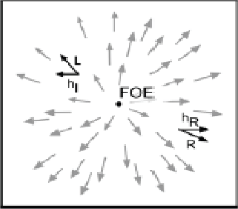
For translational motion of the camera, image motion everywhere is directed away from a singular point corresponding to the projection of the translation vector on the image plane. This point, is called the Focus of Expansion (FOE), it is computed based on the principle that flow vectors are oriented in specific directions relative to the FOE. Specifically, the horizontal component h_L of an optic flow vector L to the left of the FOE points leftward while the horizontal component h_R of an optic flow vector R to the right of the FOE points rightward, as shown in fig. 3. In a full optic flow field the horizontal location of the FOE, corresponding to the position about which a majority of horizontal components diverge (Negahdaripour, S. & Horn, K.P., 1989), can be estimated using a simple counting method to tally the signs of the horizontal components centred on each image location. At the point where the divergence is maximized, the difference between the number of h_L components to the left of the FOE and the number of h_R components to the right of the FOE will be minimized. Similarly we can estimate the vertical location of the FOE by identifying the position about which a majority of vertical components (v_U and v_D) diverge.

Fig. 3.

FOE calculation

Fig. 4 shows the result of the FOE calculation in our indoor scene, the FOE is shown by the red scare in the image.

Fig. 4.

Result of the FOE calculation

We also use the optical flow to estimate the remaining time to contact with a surface.

3.2. Time To Contact

The time-to-Contact (TTC) can be computed from the optical flow which is extracted from monocular image sequences acquired during motion.

The image velocity can be described as a function of the camera parameters and split into two terms depending on the rotational (V_t) and translational components (V_r) of camera velocity (V) respectively. The rotational part of the flow field can be computed from proprioceptive data (e.g. the camera rotation) and the focal length.

Once the global optic flow is computed, (V_t) is determined by subtracting (V_r) from (V).

From the translational optical flow, the time-to-contact can be computed by (Tresilian, J., 1990):

$$TTC=\frac{{\mathrm{\Delta }}_i}{\left|{\overrightarrow{V}}_t\right|}\dots \dots$$

(2)

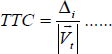
Here Δ_i is the distance of the considered point (x_i, y_i), on the image plane, from the Focus of Expansion (FOE).

Note how the flow speed, indicated by the length of the vector lines, increases with distance in the image from the focus of expansion. In fact, this distance divided by the speed is a constant, and is just the (relative) rate used to estimate time-to-contact.

In fig. 5 we show the TTC estimation of a translation sequence (a). The corresponding graph of the TTC values (b) is decreasing which is in concordance with the theory.

Fig. 5.

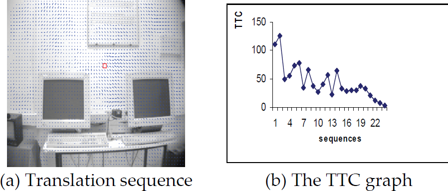
The TTC estimation

3.3. Depth calculation

Using the optical flow field computed from two consecutive images, we can find the depth information for each flow vector by combining the time to contact computation, and the robot's speed at the time the images are taken.

$$X=V.T$$

(3)

Where

X is the depth, V is the robot's speed, and T is the TTC computed for each optical flow vector.

Fig. 6 shows the depth image computed using the TTC. Darkest point is the closest while the brightest point is the farthest scene point, so the brightest zone will be the navigation zone of the robot.

Fig. 6.

Depth calculation

3.4. The Balance strategy for obstacle avoidance

The essential idea behind this strategy is that of motion parallax, when the robot is translating, closer objects give rise to faster motion across the retina than farther objects. It also takes advantage of perspective in that closer objects also take up more of the field of view, biasing the average towards their associated flow. The robot turns away from the side of greater flow. This control law is formulated by:

$$\mathrm{\Delta }(F_L-F_R)=\frac{\sum \parallel {\overrightarrow{w}}_L\parallel -\sum \parallel {\overrightarrow{w}}_R\parallel }{\sum \parallel {\overrightarrow{w}}_L\parallel +\sum \parallel {\overrightarrow{w}}_R\parallel }$$

(4)

Here Δ(F_L – F_R) is the difference in forces on the two sides of the robot's body, and $\sum \parallel \overrightarrow{w}\parallel$ , is the sum of the magnitudes of optic flow in the visual hemifields on one side of the robot's heading

We have implemented the Balance strategy on our mobile robot. As we show in fig. 7, the left optical flow (699, 24) is greater then the right one (372, 03), so the decision is to turn right in order to avoid the obstacle (the chair by the left of the robot).

Fig. 7.

result of balance strategy

4. Experimentation

The robot was tested in our robotics vision lab containing robot, office chairs, office furniture, and computing equipment. In the following experimentation we test the robot's ability to detect obstacles, using only the balance strategy.

Fig. 8 shows the view of the robot camera at the beginning of the snapshot.

Fig. 8.

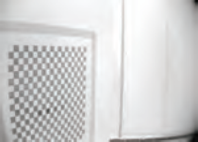
robot's view

Fig. 9(a) shows the result of the balance strategy, in which the robots have to turn right in order to avoid the nearest obstacle (the board), and fig. 9(b) shows the corresponding depth image computed from optical flow vectors, we can see that the brightest point are localised by the right of the image, so that defines the navigation zone of the robot.

Fig. 9.

First decision

Fig. 10 shows the robot's view once it turns right.

Fig. 10.

robot's view

Fig. 11 (a) shows the result of the balance strategy, in which the robots have to turn left in order to avoid the wall, and fig. 9 (b) shows the corresponding depth image in which the brightest point are localised by the left side of the image.

Fig. 11.

Second decision

Fig. 12 (c) shows the snapshot of the robot in action in our lab and fig. 12 (d) shows the path taken by the robot during this action, we notice that the robot founds 2 principal positions where it has to change orientation, the position (1) corresponding to the board and the position (2) corresponding to the wall.

Fig. 12.

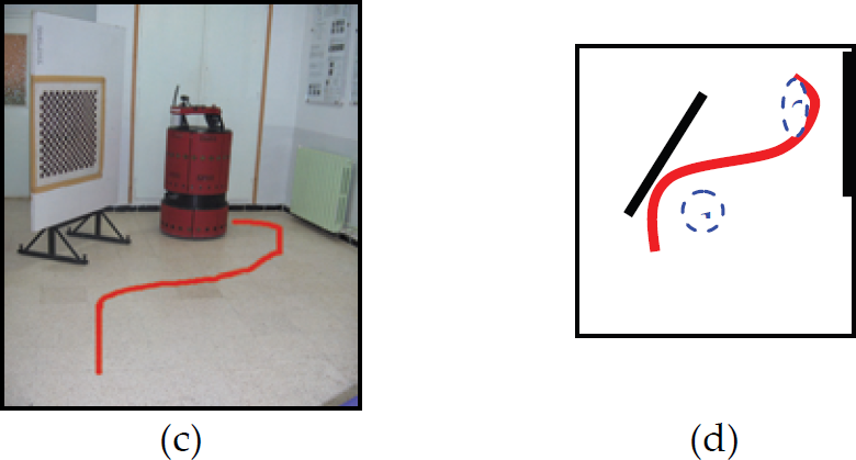
Robot in action

Fig. 13 shows the graph of both of the right and left optical flow. In the beginning of the snapshot, the left flow was greater than the right one, so the robot turns right that correspond to the position1 in fig 12 (d) then the right flow increase until it become greater than the left one because the robot became closer to the wall than to the board, we can see the intersection of the two graph (right and left flows) by the frame 5 in fig 13, and the robot turns left to avoid the wall, it correspond to the position2 in fig. 12 (d). It can be seen that the robot successfully wandered around the lab while avoiding the obstacles; however, we found that the illumination condition is very critical to the detection of the obstacle, because the image taken by the camera is more noisy in poor light conditions making the optical flow estimate more erroneous.

Fig. 13.

TTC graphe

5. Conclusion

The paper describes how, the optical flow provides a robot the ability to avoid obstacles, using the control laws called “balance strategy”, the main goal is to detect the presence of objects close to the robot based on the information of the movement of the image brightness. The major difficulty to use optical flow in navigation, is that it is not clear what causes the change of gray value? (motion vector or change of illumination). Further improvement of the developed method is possible by incorporating other sensors (sonar, infra red,…) in collaboration with camera sensor.