
Abstract
Dynamic singularities make it difficult to plan the Cartesian path of free-floating robot. In order to avoid its effect, the direct kinematic equations are used for path planning in the paper. Here, the joint position, rate and acceleration are bounded. Firstly, the joint trajectories are parameterized by polynomial or sinusoidal functions. And the two parametric functions are compared in details. It is the first contribution of the paper that polynomial functions can be used when the joint angles are limited(In the similar work of other researchers, only sinusoidla functions could be used). Secondly, the joint functions are normalized and the system of equations about the parameters is established by integrating the differential kinematics equations. Normalization is another contribution of the paper. After normalization, the boundary of the parameters is determined beforehand, and the general criterion to assign the initial guess of the unknown parameters is supplied. The criterion is independent on the planning conditions such as the total time tf. Finally, the parametes are solved by the iterative Newtonian method. Modification of tf may not result in the recalculation of the parameters. Simulation results verify the path planning method.
Introduction
Robotic systems are expected to play an increasingly important role in the future space activity. One broad area of application is in the servicing, construction, and maintenance of satellites and large space structures in orbit. However, the planning and control of the robotic manipulators pose additional problems beyond those on earth, due to the dynamic coupling between space manipulators and their spacecraft. Free-floating systems exhibit nonholonomic behavior, which results from the non-integrability of the angular momentum. The free-floating mode is very important, since it can save the fuel of the spacecraft and avoid collision.
There are many literatures dealing with the problem of the path planning for free-floating space robot. Z. Vafa and S. Dubowsky (Vafa, Z. & Dubowsky, S. 1990) proposed cyclic motion of the manipulator joints to change the vehicle orientation. However, this scheme has to assume small cyclic motion to neglect the nonlinearity of order greater than two, and it requires many cycles to make even a small change of vehicle orientation. Y. Nakamura and R. Mukherjee (Nakamura, Y. & Mukherjee, R. 1991) discussed the nonholonomic characteristics of free-floating space manipulators, and employed “bidirectional approach” for path generation aiming at controlling both the manipulator configuration and the spacecraft orientation. Although of much success, the control law failed to achieve some desired orientations and smooth feedbacks didn't exist. T. Mineta et al. planned the trajectory of a space manipulator using a neural network (Mineta, T., J. Qiu and Tani, J. 1997). K. Yamada (Yamada, K. 1993) used the variational method to find a closed trajectory of manipulator joints that generates an arbitrary change of satellite attitude. T. Suzuki and Y. Nakamura (Suzuki T. and Nakamura Y. 1996) extended Yamada's method to obtained the optimal spiral motion, which is considered an approximation of an arbitrary given 9-dimensional trajectory of the end-effector pose and the satellite orientation. The “spiral motion” planning method is a good attempt, but its convergence is affected by the singular point. C. Fernandes et al (Fernandes, C., Gumits, L., and Li, Z.X. 1994) developed a near-optimal path planning approach for controlling the spacecraft attitude and manipulator posture at the same time using internal motion. The approach didn't assume any specific structure of a system and can be automated computationally, but it needs symbolic manipulation software to obtain the Jacobians required by the algorithm. M. Torres and S. Dubowskys (Dubowsky S., Torres M. 1991) presented a technique called the Enhanced Disturbance Map (EDM) to plan space manipulator motions that will result in relatively low spacecraft disturbances. But the EDM is not easy to attain, especially for the space robotic system of higher degree of freedom. K. Yoshida et al. (Yoshida, K., Hashizume, K. and Abiko, S. 2001) addressed the Zero Reaction Maneuver (ZRM) concept, but the existence of ZRM is very limited for a 6 DOF manipulator. K. Yoshida et al. (Yoshida, K., Kurazume, R. and Umetani, Y. 1991) proposed that one of the manipulators of a free-flying system should move to compensate for the disturbance created by the other. It is a useful method but will augment the cost of the project and the complexity of the cpntrol algorithm.
Path planning of free-floating robot in Cartesian space belongs to the problem of “Inertially-Referenced End-Point Motion Control”(Papadopoulos, E. and Dubowsky, S. 1991). In the case of inertial manipulation, such as capturing a free object in space, some control methods based on Generalized Jacobian Matrix (GJM) can be used. These methods include resolved rate, resolved acceleration or transposed Jacobian control technology. But the algorithms that use a Jacobian inverse, such as the resolved rate or resolved acceleration control algorithms, fail at dynamic singularities. Ones that use a pseudo inverse Jacobian or a Jacobian transpose will likely follow the available direction, but they may result in large errors.
Dynamic singularities are path dependent (Papadopoulos, E. and Dubowsky, S. 1993). Based on the calculation of PIW (Path Independent Workspaces) and PDW (Path Dependent Workspace), E. Papadopoulos (Papadopoulos, E. 1992) proposed a planning algorithm that avoids dynamic singularities, and it permits the manipulator's end-effector to move from any reachable workspace location to any other. But Papadopoulos only took a planar 2-link robot as the example. In fact, the calculation of PIW and PDW of a space manipulator of higher degree of freedom is very complicated. S. Pandey (Pandey, S. and Agrawal, S. 1997) proposed a method called “mode summation” to plan the Cartesian path of a free-floating system with prismatic joints. R. Lampariello et al. (Lampariello, R. and Deutrich, K. 1999) applied the method to a system with rotational joints. But they used sinusoidal functions to satisfy the limits of the joint variables, since they thaught polynomial functions could not attain the aim. The method to solve the problem of path planning, which is an iterative method, requires to assign the initial values of the unknown parameters. R. Lampariello et al. developed a criterion to do so. The criterion depends on certain condition, such as the planning time tf. Therefore, it needs recalculating if the condition changes. Moreover, they didn't propose a general method to take the limit of joint rate and acceleration in the planning problem. In this paper, the method is improved to tackle these problems. Polynomial and sinusoidal functions can be used in the case that the joint position, rate and accelaration are bounded. Furthermore, the boundary of the parameters can be determined beforehand and a general criteria is proposed to assign the initial values of the parameters. Modification of tf can't result in the recalculation of the parameters.
This paper is organized as follows: Section two derives the kinematic equations of space robotic system. Then, the problem of Cartisian path planning is discussed in Section three. In Section four, the joint functions are parameterized and normalized to solve the path planning problem. In Section five, the simulation results are showed. Section six is for conclusion and discussion. The last section is the acknowledgement.
Modelling of Free-Floating Robotic System
Major research topics on space robot dynamic and control were collected by Xu and Kanade(Xu, Y. S. and Kanade, T. 1992). Fig.1 shows a general model of a space robot system with a single manipulator arm, which is regarded as a n+1 serial link system connected with n degree of freedom active joints. B0 denotes the satellite main body, Bi (i = 1, …, n) denotes the ith link of the manipulator, and Ji is the joint which connects Bi−1 and Bi.

General Model of a Single Arm Space Robot
Some symbols and variables are defined as follows:
Σ
I
: the inertia frame; Σ
E
: the frame of the end-effector; Σ
i
: the frame of Bi; Ci(i = 0, …, n): the CM (center of mass) of Bi Si, bi ∈R3: the position vectors from Ji to Ci and Ci to Ji+1 respectively; ψ
b
, ψ
e
∈ R3: the attitude angle of the base and the end-effector respectively, expressed in terms of x-y-z Euler angles, i.e. ri ∈ R3: the position vectors of Ci; pe ∈ R3: the position vectors of the end-effector; Θ ∈ Rn : the joint angle vector, Θ=[θ1, …, θn];
The direct kinematics of space robot system is in the form as follows(Umetani, Y. and Yoshida, K. 1989):
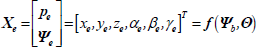
where, Xe is the pose (position and orientation) of the end-effector. For an n joint manipulator, the system of equations (1) has n equations but n+3 unknowns, so it can not be solved. It is easy to deduce from this result that the path planning method which makes use of the non-differential form of the kinematical equations of the system is not suitable for free-floating systems.
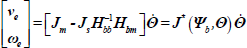
The differential form of the kinematical equations of space robot system is:

where

where Hbb∈R6×6 is the inertia matrix of the base and Hbm∈R6×n is the coupling inertia matrix. From equation (3), vb and ωb are solved as:

where, Jvb and Jwb are the Jacobian matrices relating
The matrix
When the orientation is expressed in x-y-z Euler angles, the relationship between the resolute angle velocity and the Euler angle velocity is given by:
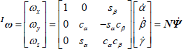
where,


Therefore, the differential kinematical equation of the free-floating system becomes:
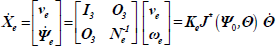
where, I3 is a 3×3 identity matrix and O3 is a 3×3 zero matrix. Ke is the composite matrix, i. e.

Description of the Problem
Point-to-point path planning in Cartesian space for free-floating space robot is studied in the paper, i. e., joint path is planned to make the end-effeor attain the desired pose Xed. The following equations are obtained by integrating the equation (7) and (9):
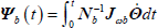
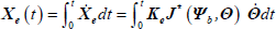
The integral can not be gotten analytically, but it can be calculated numerically. Then the problem of the path planning is expressed as follows:
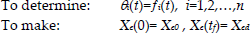
Subject to the equality constraints:

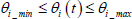
and the inequality constraints:
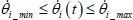
In order to solve the problem of the path planning, the joint functions are parameterized here. There are two methods for the parameterization: one is polynomial parameterization, the other is sinusoidal parameterization. Each has its own advantages, which will be discussed.
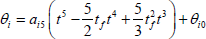
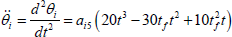
S. Pandey et al. used polynomial functions to parameterize the manipulator joints when there are no limits on the manipulator joints(Pandey, S. and Agrawal, S. 1997). The degree of the function must satisfy the constraints on the position, velocity and acceleration of the joints. According to the condition of (13), a polynomial functions of fifth degree can be used for the parameterization of ith joint, i. e.

where, 0<t<tf, and ai0 ˜ ai5 are the coefficients of the polynomial. Applying the equality constraints of Equation (13) to Equation (17), the following results are found:


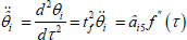
Correspondingly, the joint position, velocity and acceleration functions are given by:
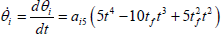
Therefore, there is only a parameter a
i5
in each joint function after parameterization. If n=6, let a=[a15,a25,…,a65]. Then the difference between Xed and Xef is the function of a too, i.e.

The path planning problem is reduced to the resolution of the system of nonlinear equations as follows:

when the parameter a is solved, the joint path is determined.
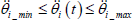
The joint positions can be limited between a maximum and a minimum value, for reasons of mechanical or operational nature. That is to say, the joint functions must satisfy the constraints of (14). Since sinusoidal functions are bounded, they are used here to parameterize the joint angle functions, which is similar with the methods of S. Pandey's and R. Lampariello's(Pandey, S. and Agrawal, S. 1997; Lampariello, R. and Deutrich, K. 1999). The arguments of the sinusoidal functions are polynomial functions. The parameterized joint functions are
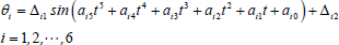
where, 0≤t≤tf and ai0 ˜ ai5 are the coefficients of the polynomial. Δ
i1
and Δ
i2
are defined as

where, Θ
imin
and Θ
imax
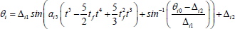
are the minimum and maximum of ith joint. Applying (13) to (27), the coefficents can be solved:


Therefore, the joint position, velocity and acceleration functions are shown as the following equations:
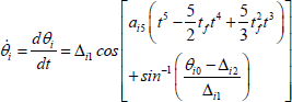

There is only a parameter ai5 in each joint function after parameterization, too. For the case of n=6, let a=[a15,a25,…,a65]. Then Equations (25) and (26) are also given.
R. Lampariello (1999) and S. Pandey (1997) used sinusoidal functions to paraterize the joint functions when the constrints on joint angles were considered. And the unknown parameters were solved by iterative Newtonian method. R. Lampariello (1999) proposed a criteria for assigning the initial guess of the unknown parameters. But the initial guess is dependent on the total time tf, therefore, it is not of generality.
Here we proposed a modified method to tackle these problems. Some work is reported on the cofference RA 2005 (Xu, W. F., Liang, B., Ti, C. et al. 2005). With the method, both polynomial and sinusoidal functions can be used to plan the joint motion for the case that joint position, rate and acceleration are limited. And a more practicable criteria is developed to assign the initial values of the unknown parameters, which guarantees that the path solved is the preferable path when there are more than one path, and that the parameters converge even if the manipulator needs a long range manoeuvres. The key of the method is the normalization of the joint functions.
Normalization of the Polynomial Functions
Let

where,

Similarly, the joint rate and acceleration function with respect to the normized time τ are as follows:

The integrals and the corresponding system of nonlinear equations are
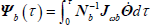


Then the path planning problem becomes the problem to solve the parameter
The curves of f(τ) and its first and second derivatives are shown as Fig. 2.

f(τ) and Its First and Second Derivatives
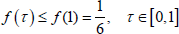
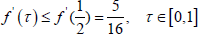
It is obvious that f(τ) increases monotonously between [0,1]. The bounds of f(τ) and its first and second derivatives are calculated as follows:

According to Equations (14), (36) and (43), the parameter

Inequalities (46) can be written in the vector form as
Moreover, tf can be used to limit joint rate and acceleration. According to Equations (15), (16), (38), (39), (44) and (45), the total time of the path planning is determined according to the following inequalities.


When the solved parameter
Similaly, sinusoidal joint functions can be normalized. Let


The joint function with respect to time for different parameter values are shown as fig.3 (assume that θ i ∈[−140°, 170°]). Different from the case of polynominal functions, the joint functions are highly nonlinear with respect to the parameter a. And the joint angle is always within the upper and lower bounds.

Joint Function with respect to time for different values of the parameter ai5
The system of the equations with respect to the unknown parameters can be solved with an iterative Newtonian method. The algorithm is as follows:
Initialization: Xef is gotten by integrating the Equation (41) and if k=k+1, go to 2); if Output the parameter


The whole processs is shown as Fig.4

The Flow-Chart of the Algorithm
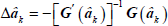
The final pose of the end-effector Xef is a hypersurface of the parameter â. Fig.5 indicates the variation of Xef with the parameter
Pose of the End-effector vs Parameter a15
For the case of sinusoidal parameterization, the variation of Xef with the parameter can be analyzed in the same way as the case of polynominal parameterization. It shows that when

Final Value with respect to the parameter ai5
There are some advantages of the path planning method proposed in the paper:
Not only sinusoidal functions but also polynomial functions can be used to plan the Cartesian path when the limits on joint angles, rates, accelerations are considerd. The boundary of the parameters can be defined beforehand. Therefore, the resolution algorithm only needs to search the parameter withen the boundary, which simplifies the algorithm. A general criteria is supplied to assign the initial guess of the unknown parameters, which is independent on the planning conditions such as the time tf. A general method is proposed to take the constraint on joint angles, rates and accelerations in the solution to the problem of the path planning.
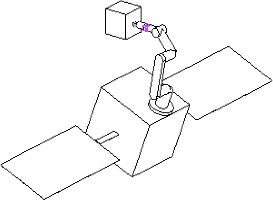
Space Robotic System
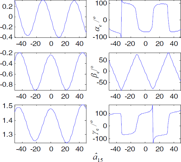
A space robot system is composed of a spacecraft, a 6 DOF manipulator mounted on the spacecraft and an object as a target to be captured by the manipulator, as Fig.7. The body-fixed frames of the space robotic system are defined by Denavit-Hartenberg convention, as Fig.8. The base frame, which is fixed on the satellite, and the ith body frame are represented by Σ0 and Σ
i
respectively. The Denavit-Hartenberg parameters of the manipulator are given in Tab.1. And Tab.2 shows the CM position vector


A Space Robotic System
The D-H Coordinate System
D-H Parameters of the Manipulator

The CM and Mass Properties of Each Body

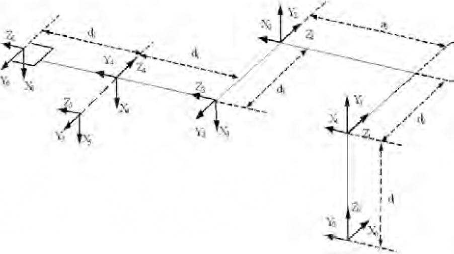
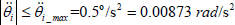
Not loss of generality, the limits on the joint velocity and acceleration are assumed to be:
For the point-to-point manoeuvre as Fig.7, the initial and desired pose of the end-effector are as follows:

The initial values of the manipulator joints and the satellite attitude are Θ0 =[π/2,0.32, −0.14, 0, 0.6, π]
T
) and ψ
b
(0)=[0,0,0]T respectively. According to the criterion proposed above, the initial guess of the parameter 
The convergence error is

Then the total time tf must satisfy the following inequalities (according to (47) ˜ (48)):


At last, tf is chosen as tf=30.2. According to the simulation results, the planned joint angles and the corresponding attitude change of the base are shown as Fig.9. And the joint rate and acceleration vary as Fig.10 and Fig.11 respectively. They are within their bounds. In order to verify the planned path, the dynamic model of the whole system is created by ADAMS–a powerful mechanical motion simulation software (MSC software. 2005). The joint data (θ1˜θ6) are imported to ADAMS, and the dynamic simulation is done. The final state of the simulation is shown as Fig.12. It can be seen that the pose of the end-effector attains the desired pose although the orientation of the base changes largely.

The Joint Angles and the Attitude of the Satellite
The Manipulator Joint Angle Velocities

The Manipulator Joint Angle Accelerations
The State of the System after Point-to-Point Manoeuvre
The simulation condition is the same as that of the case of sinusoidal parameterization. According to the criterion, the initial value of the parameter 
The convergence error is

The total time is determined by the following inequalities
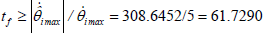
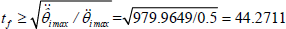
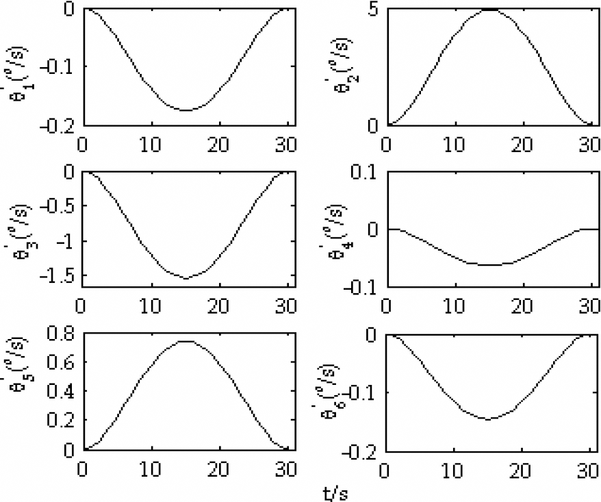
Therefore, the total time is choosen as tf=62s. According to the simulation results, the variation of the manipulator joint angles and the base attitude are shown as Fig.13. And the joint rate and acceleration vary as Fig.14 and Fig.15 respectively.
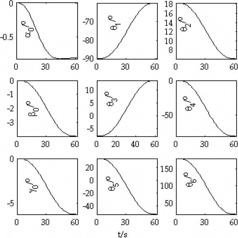
Joint Angles and Satellite Attitude

The Manipulator Joint Angle Velocities
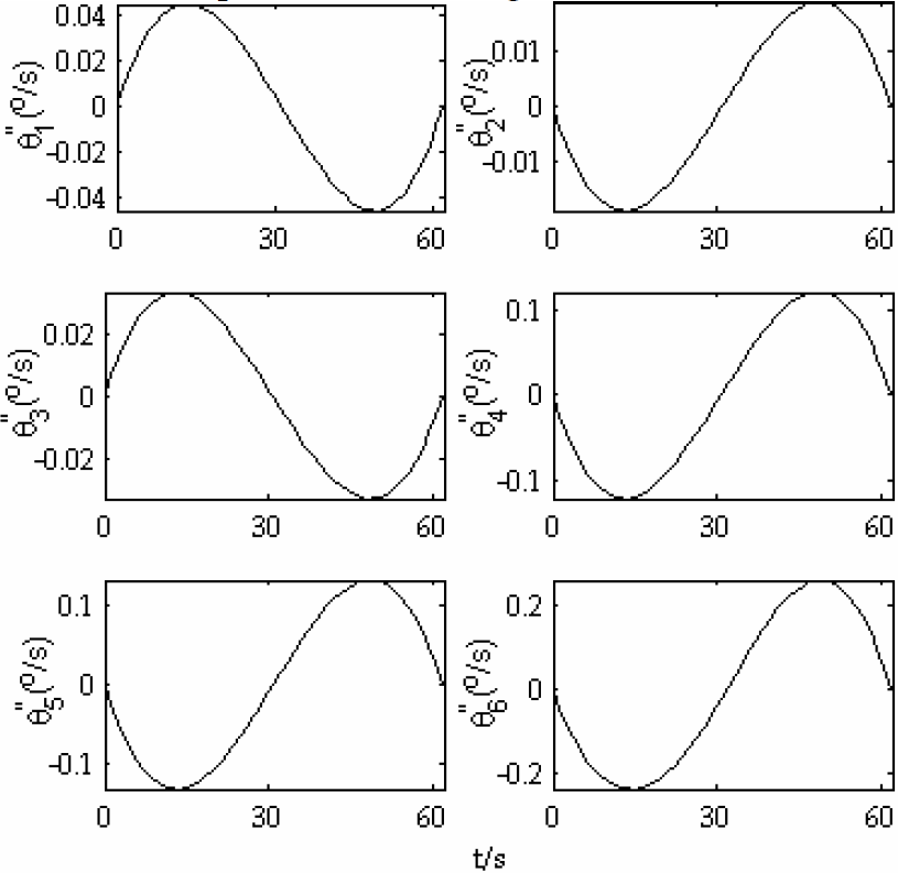
The Manipulator Joint Angle Accelerations
Direct kinematic equations are used to plan the Cartesin path of free-floating robot, which is a good way to avoid the effect of dynamic singularies. The key of the method is the normalization of the parameterized functions of the manipulator joints. Polynomial and sinusoidal parameterized functions have their own advantages. Sinusoidal functions are used to limit joint angles direcly, but the convergence time is longer than that of the case of polynomial parameterization. After normalization, polynomial parameterization is more effective than sinusoidal parameterization since the constraints are easy to satisfied. So we suggest to use polynomial function to parameterize the joint angles. Moreover, it is worth pointing out that Euler angles are not globally singularity-free representation of the attitude, so the unit quaternion shouled be used when the variation of attitude is possibly larger that π/2.
The shortcoming of the method is that the convergence time is long. Furtherover, there are different paths to reach the desired pose of the end-effector because of the nonholonomic redundancy of the free-floating system. Therefore, the future research will focus on optimal plan based on some cost functions. The path planning for attitude variation using the manipulator joints is another interest. At the same time, we will try to improving the efficiency of the algorithm.
Footnotes
7.
We would like to thank Dr. L.T. Li and Dr. Y. Liu for their valuable suggestion on the paper. This work is supported by Chinese High-Tech Program in Aerospace.