
Abstract
The Cartesian path planning of free-floating space robot is much more complex than that of fixed-based manipulators, since the end-effector pose (position and orientation) is path dependent, and the position-level kinematic equations can not be used to determine the joint angles. In this paper, a method based on particle swarm optimization (PSO) is proposed to solve this problem. Firstly, we parameterize the joint trajectory using polynomial functions, and then normalize the parameterized trajectory. Secondly, the Cartesian path planning is transformed to an optimization problem by integrating the differential kinematic equations. The object function is defined according to the accuracy requirement, and it is the function of the parameters to be defined. Finally, we use the Particle Swarm Optimization (PSO) algorithm to search the unknown parameters. The approach has the following traits: 1) The limits on joint angles, rates and accelerations are included in the planning algorithm; 2) There exist not any kinematic and dynamic singularities, since only the direct kinematic equations are used; 3) The attitude singularities do not exist, for the orientation is represented by quaternion; 4) The optimization algorithm is not affected by the initial parameters. Simulation results verify the proposed method.
Introduction
Robotic systems are expected to play an increasingly important role in the future space activity. One broad area of application is in the servicing, construction, and maintenance of satellites and large space structures in orbit. However, the planning and control of space robot pose additional problems beyond those on earth, due to the dynamic coupling between space manipulators and their spacecraft (Nakamura & Mukherjee, 1991; Xu et al., 2006; Huang et al., 2006). Free-floating systems (Both the attitude and position of the base are not controlled) exhibit non-holonomic behavior, which results from the non-integrability of the angular momentum. The free-floating mode is very important, since it can save the fuel of the spacecraft and avoid collision. So, many scholars have been studing the planning and control of free-floating space robot. Huang et al presented a minimum-torque path-planning scheme in joint space (Huang et al., 2006). For inertial manipulation, such as capturing a free object, some methods based on Generalized Jacobian Matrix (GJM) are proposed (Umetani & Yoshida, 1989; Moosavian & Papadopoulos, 1997; Moosavian & Papadopoulos, 2007; Traira et al., 2000). However, the algorithms that use a Jacobian inverse, such as the resolved rate or resolved acceleration control algorithms, fail at dynamic singularities. Ones that use the pseudo inverse or transpose of the Jacobian will likely follow the available direction, but they may result in large errors.
Dynamic singularities are path dependent (Papadopoulos & Dubowsky, 1993). Based on the calculation of PIW (Path Independent Workspaces) and PDW (Path Dependent Workspace), Papadopoulos (Papadopoulos, 1992) proposed a planning algorithm that avoids dynamic singularities, and permits the manipulator's end-effector to move from any reachable workspace location to any other. But the PIW and PDW's calculation for a space manipulator of higher degree of freedom is very complicated. Papadopoulos and Tortopidis also developed a path planning methodology that allows simultaneous manipulator end-point and spacecraft attitude control using manipulator actuators only (Papadopoulos et al., 2005; Tortopidis & Papadopoulos, 2007). Pandey (Pandey & Agrawal, S., 1997) proposed a method called “mode summation” to plan the Cartesian path of a free-floating system with prismatic joints. Lampariello et al. (Lampariello & Deutrich, 1999) applied the method to a system with rotational joints. But they didn't propose a general method to limit the joint accelerations. They also did not develop a general criterion to assign the initial values of the unknown parameters. The authors (Xu et al., 2007) improved the mxethod to tackle these problems, by normalizing the joint functions. However, there are still some shortcomings of the method. Firstly, the essential of the method is a Newton iterative algorithm, which will converges to local minimum. Secondly, the initial parameters are very important for the convergence speed. If they are assigned close to the solutions, the convergence speed is quadratic. Otherwise, the algorithm converges very slowly. Thirdly, the representation of the body attitude (including the base attitude and the end-effector attitude), which is described by Euler angles, will meets with singular orientations (i.e. the Jacobian that maps differential changes in the representation to the angular velocity is singular for some orientations). In this paper, an approach, which is the further research of the previous work (Xu et al., 2007), is proposed to plan the Cartesian plan of free-floating space robotic system. The system is composed of a 6 DOF manipulator and a satellite. The method solves the shortcomings of the old algorithm.
This paper is organized as follows: Section two derives the kinematic equations of space robotic system. Then, the problem of Cartesian path planning is discussed in Section three. In Section four, the joint functions are parameterized and normalized, and the PSO algorithm is used to solve the path planning problem. In section five, the simulation results are showed. Section six is for conclusion and discussion. The last section is the acknowledgement.
Modeling of Space Robotic System
Symbols and Variables
Major research achievements on space robot were collected by Xu and Kanade (Xu & Kanade, 1992), and were also reviewed by Moosavian and Papadopoulos recently (Moosavian & Papadopoulos, 2007).
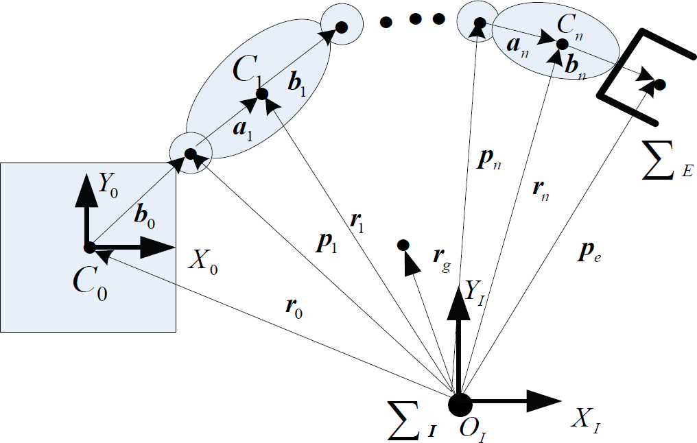
Here, we model the space robotic system using Lagrangian method. Fig.1 shows a general model of a space robot system with a single manipulator arm, which is regarded as a n+1 serial link system connected with n degree of freedom active joints. B0 denotes the satellite main body, B i (i = 1, …, n) denotes the i th link of the manipulator, and J i is the joint which connects B i-1 and B i . In order to conveniently discuss, some symbols and variables are defined as follows (The following vectors are described in the inertia frame, if not pointed out specially):
General Model of a Single Arm Space Robot
Σ I , Σ E : the inertia frame and the end-effector frame, respectively;
Σ i (i = 0, …, n): the body fixed frame of B i
C i (i = 0, …, n): the position of the B i 's centroid
m i (i = 0, …, n): the mass of B i ;
M: total mass of the system, i.e.
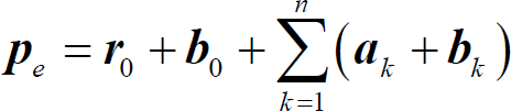
From Fig. 1, the position vector of the end-effector is
Differentiating it with respect to time, a relationship between end-effector linear velocity and joint velocity is obtained, i.e.

On the other hand, a relationship between end-effector angular velocity and joint velocity is expressed with

Then, the differential kinematic equation can be determined according to (2) and (3), i.e.:

where, J
b
and J
m
are the Jacobian matrixes dependent on the base and the manipulator, respectively(see Ref. (Yoshida, 2003)). Since no external forces and torques acting on the free-floating system, the linear and angular momentums are conserved. With the assumption that their initial values are zeros, the momentum conservation equations of the free-floating space robot are
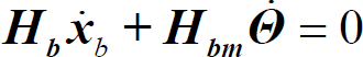
The matrixes H
b
and H
bm
, whose expressions can be found in Ref. (Yoshida, 2003), are the inertia matrix of the base and coupling inertia matrix, respectively. Then

The matrix J
bm
is base-manipulator Jacobian matrix and J
bm_v
and J
bm_ω
are its sub matrixes. Substituting (6) to (4), the kinematic equations of free-floating space robotic system are given as

where,
Euler angles are the common minimal representation of attitude. However there are always singular orientations. For example, if the attitude is represented by the Z-Y-X Euler angles

When
However, when β = ±π/2,
The unit quaternion is a popular nonsingular four-parameter representation(Jack, 1992). A quaternion

where, r and Ψ are, respectively, the unit vector and the rotation angle of an equivalent angle/axis description. Notice that, the scalar part and the vector part are constrained by

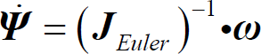
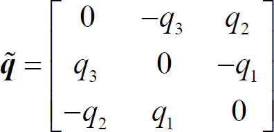
It is well known that {η, q} and {-η, -q} represent the same orientation. In this paper, Ψ is bounded by (−π, π], so η≥0. The relationship between the time derivative of the quaternion and the angular velocity is established by

where,
For two coordinate systems, if their orientations are represented by {η, q1} and {η2, q2} respectively, the relative attitude is given by {Δη, Δq}, where (Yuan, 1988)

When the two frames coincide,

Furthermore, through the normality condition (11), δq=0 implies δ, η=±1. Therefore, it can be concluded that the two frames coincide if and only if δq=0.
The space robotic system studied in the paper is shown as Fig. 2. It is composed of a carrier spacecraft (called Space Base or Base), a PUMA-type manipulator (called Space Manipulator) and a target satellite (called Target to be captured. The frames fixed on the multi-body system are defined as Fig. 3 (when the joint angles are all zeros), where Z
i
is the direction of J
i
and the link lengths are denoted by L1∼L7. Table I lists the dimensions and mass properties of the bodies (Sat and B
i
stand for the satellite and the ith body, respectively). The link vectors
i

The space robotic system studied in the paper

The body-fixed frames of the space robotic system
The Mass Properties of the Space Robotic System

Description of the Problem
Point-to-point path planning in Cartesian space for free-floating space robot is studied here, i.e., the joint path is planned to make the end-effeor attain the desired pose. Then, the system state is composed of the attitude (quartenion) and position of the end-effector:

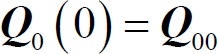
Equation (16) shows that, the end-effector is the function of the base attitude and the joint angles. Correspondingly, the initial, final and desired poses of the end-effector are written as 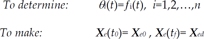
subject to the equality constraints:

and the inequality constraints:
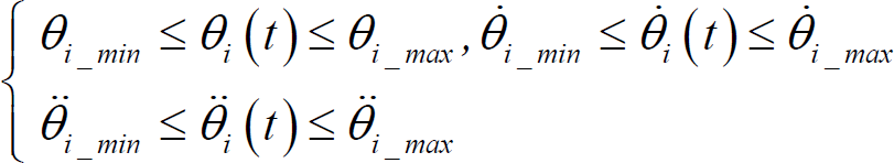
where, 
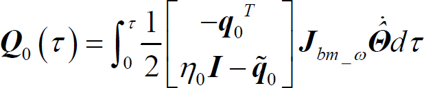
According to Equations (6), (7) and (12), the following results are given
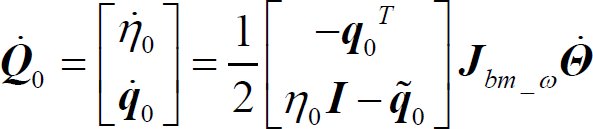
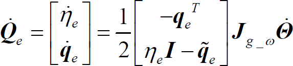
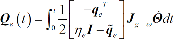
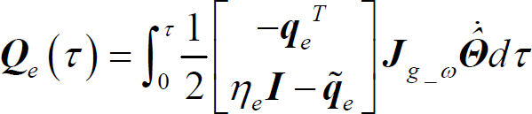
Therefore, the base attitude and end-effector attitude at time t are obtained by the integrals:

Then, From Equation (14), the orientation difference of end-effector at time t
f
is:

where, {ηef, q
ef
} and {η
ed
, q
ed
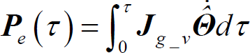
} are the quaternion representations of the final and desired values of the end-effector orientation. On the other hand, the end-effector position is given by the integral (see Equation (7)):

And the position difference of end-effector at time t
f
is:

The polynomial functions are usually used to get smooth joint motion(Angeles, 2006). Here we parameterize the joint angle by 5th order polynomial functions:
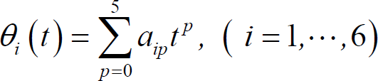
where, 0≥t≥t
f
, and ai0∼ai5 are the coefficients of the polynomial. Applying the constraints of Equation (17) to Equation (28), the results are:
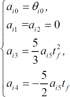
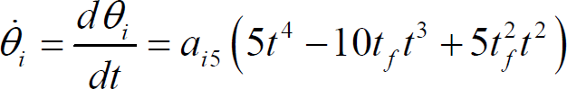
Correspondingly, the joint position, velocity and acceleration functions are given by:
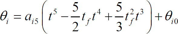

From (30)∼(32), there is only a parameter ai5 in each joint function after parameterization. Let

when the parameter 
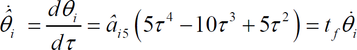

where,

Correspondinly, the integrals (23), (24) and (26) become
And, known from (25) and (27), the end-effector pose error at t
f
is the function of the parameters 
According to (20) and (41), the planning problem can be transformed to an optimization problem, whose object function is defined according to the accuracy requirement. A good choice is
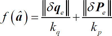
where, the norm ‖x‖ = x
T
x, and, k
q
and k
p
are the weight parameters of attitude error (represented by quaternion) and position error, respectively. Then, the planning problem is reduced to the searching of the optimized parameter

Object function Calculation
Review of Particle Swarm Optimization
Particle Swarm Optimization (PSO), which resembles a school of flying birds, was originally developed by Kennedy and Eberhart to efficiently find optimal or near-optimal solutions in large search spaces (Kennedy & Eberhart, 1995; Eberhart & Kennedy, 1995). In a particle swarm optimizer, instead of using genetic operators, these individuals are “evolved” by cooperation and competition among the individuals themselves through generations. Each individual, named as a “particle”, adjusts its flying according to its own flying experience and its companions' flying experience. It represents a potential solution to a problem, and is treated as a point in a n-dimensional space. The ith particle is described as

The best previous position (the position giving the best fitness value) of any particle is recorded and written as

and the best particle among all the particles in the population is denoted by
The velocity of particle i is

Then, the particles are manipulated according to the following equations (Shi and Eberhart, 1998):

where, c1 and c2 are two positive constants, called the cognitive and social parameter respectively; rand() and Rand() are two random functions in the range [0,1]. The inertia weight w plays the role of balancing the global search and local search. It can be a positive constant or even a positive linear or nonlinear function of time. The particle swarm optimizer has been found to be robust and fast in solving nonlinear, non-differentiable, multi-modal problems.
One of the reasons that particle swarm optimization is attractive is that there are very few parameters to adjust. It has been used for the path planning of free-floating space robot (Huang & Xu, 2006) and underactuated runing robot (Takahashi et al., 2006). Here, the optimization problem of (42) is solved using the PSO algorithm too. Firstly, the ith particle is defined as
The population size is assumed to be n
p
, and the maximum number of iterations (epochs) to train is N
max
. The iteration number is denoted by k. Then, the optimization procedure is as follows:
Set k=1, and initialize a population (array) of particles with random positions and velocities on n dimensions(here, n=6) in the problem space:
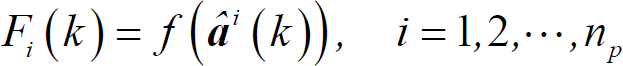
The fitness function of each particle F
i
is calculated by (42), i.e.
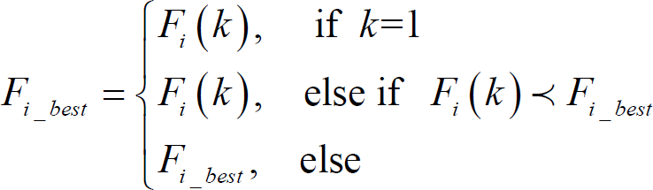
To calculate the best previous fitness evaluation of each particle F
i_best
and the best previous position 4. To calculate the best fitness evaluation F
g_best
and the best particle where, Change the velocity and position of the particle according to equations (47) and (48), respectively: Loop to step 2) until a criterion is met, usually a sufficiently good fitness or a maximum number of iterations (N
max
).


The whole process of the algorithm is shown as Fig.5. Particles' velocities on each dimension are limited to a maximum velocity Vmax. If the sum of accelerations cause the velocity on that dimension to exceed Vmax, which is a parameter specified by the user, then it is assigned as Vmax. Therefore, Vmax is an important parameter. It determines the resolution, or fineness, with which regions between the present position and the target (best so far) position are searched. If Vmax is too high, particles might fly past good solutions. If it is too small, on the other hand, particles may not explore sufficiently beyond locally good regions. In fact, they could become trapped in local optima, unable to move far enough to reach a better position in the problem space.

The Flow-Chart of the Algorithm
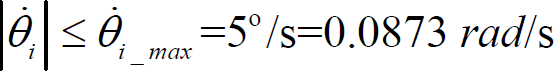
Not loss of generality, the limits on the joint velocity and acceleration are assumed to be:

The initial and desired poses of the end-effector are


The initial values of joint angles (

The object function is defined as (42). If the admitted orientation error and position error are 1° and 5 mm respectively, k
q
and k
p
are determined as


After the normalization, the bound of âi5 can be set (Xu et al., 2007)
The parameters for the algorithms are:

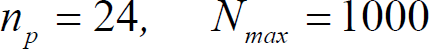


The inertia weight w is decreased linearly from wmax to wmin during a run. The converged parameters and the corresponding object function are (The convergence process is shown as Fig. 6.)

The Variation of the Global Best Fitness Evaluation
The total time is determined by (Xu et al., 2007)


Therefore, it is chosen as t f =20s. According to the simulation results, the planned joint angles are shown as Fig. 7. And the joint rate and acceleration vary as Fig. 8 and Fig. 9 respectively. These trajectories are very smooth and suitable for the control of the manipulator. The curves of the end-effector orientation and the position are shown as Fig. 10 and Fig. 11. Both show that, the end-effector moves from the initial pose to the desired pose. The corresponding attitude of the base changes as Fig. 12.

The Planned Joint Angles

The Curves of Joint Rates during the maneuver

The Curves of Joint Accelerations during the maneuver

The Curves of the End-effector Attitude Quaternion

The Curves of the End-effector Position

The Variation of the Base Attitude (represented by Quaternion)
For free-floating space robotic system, the end-effector pose is not only dependent on the current joint angles, but also on the history of each joint path. Therefore, the position-level kinematic equation can not be used to plan the Cartesian path, although it is often used by the fixed-based manipulators. In this paper, we propose an approach to plan the Cartesian point-to-point path. After parameterization and normalization of joint trajectories, the planning problem is transformed to an optimization problem, and the PSO algorithm is used to search the parameters to be determined. It is more applicable, since the constraints on the joint angles, rates and accelerations are included into the planning method, and the planned path is very smooth to control the manipulator. Furthermore, the kinematic and dynamic singularities do not affect the algorithm, because only the direct kinematic equations are used. Another advantage is that the convergence of the algorithm is not affected by the attitude singularity, for the orientation error is represented by quaternion. And the initial parametesr have little effect on its convegence.
It is worth pointing out that the reason of parameterization using monotonic functions is for the possible shorter manoeuvre, not especially for the PSO. If the desired poses is infeasible (such as the poses beyond the workspace), the PSO will search the parameters generating the minimum differences between the final poses and the desired poses. The shortcomings of the algorithms are: 1) The accumulated error in the numerical integration will affect the accuracies of the position and attitude of the end-effector; and 2) the computational cost might be large and the convergence time will be long. The future work will focus on the improving of the algorithm.
Footnotes
7.
We would like to thank Dr. P. F. Huang and Dr. L. T. Li for their valuable suggestion on the paper. This work is supported by National Nature Science Foundation of China (No.60775049).