
Abstract
In this paper, we introduce a new method and new motion variables to study kinematics and dynamics of a 6 d.o.f cable-driven robot. Using these new variables and Lagrange equations, we achieve new equations of motion which are different in appearance and several aspects from conventional equations usually used to study 6 d.o.f cable robots. Then, we introduce a new Jacobian matrix which expresses kinematical relations of the robot via a new approach and is basically different from the conventional Jacobian matrix. One of the important characteristics of the new method is computational efficiency in comparison with the conventional method. It is demonstrated that using the new method instead of the conventional one, significantly reduces the computation time required to determine workspace of the robot as well as the time required to solve the equations of motion.
Introduction
Cable-driven robots or cable robots are a special form of parallel robots in which the rigid links are replaced by cables. These robots have desirable advantages over parallel robots such as large workspace, low inertia properties, high payload-to-weight ratio, transportability, reconfigurability and economical construction. On the other hand, the main disadvantage of cable robots is that cables are only capable of pulling and it can cause instabilities in their motion. Several cable robots have been studied in the past. An early robot is the Robocrane (Albus, J. et al., 1993) developed by NIST for use in shipping ports. Another cable robot is Charlotte (Campbell, P. et al., 1995) developed by McDonnell-Douglas for use on International Space Station. The other cable robots which have been built and tested are: the Texas (Lindemann, R. & Tesar, D., 1989), and the FALCON (Kawamura, S. et al., 1995).
Workspace is as an important issue in cable robots and has been studied by many researchers. Fattah and Agrawal studied the optimal design of Planar Cable Robots (Fattah, A. & Agrawal, S., 2002). Barrette and Gosselin analytically determined the dynamic workspace of a planar cable robot (Barrette, G. & Gosselin, C., 2005). Although it is desirable to obtain workspaces by analytical methods, but because of inherent complexity in cable robots, such methods can be used only for planar robots and simple geometries. On the other hand, numerical methods have fewer limitations and are usually used by researchers. One of the disadvantages of numerical methods is that they need an exhaustive and time-consuming search in the entire taskspace. Alp and Agrawal determined the statically reachable workspace for a 6 d.o.f spatial cable robot which has been built and tested in University of Delaware (Alp, A. & Agrawal, S., 2002). They created a three dimensional grid and searched in this volume. Pusey also used exhaustive search to determine the workspace of a 6 d.o.f cable robot (Pusey, J. et al., 2004).
In this paper, using the concept of kinematic constraints and Lagrange method, a new Jacobian matrix and a new form of equations of motion for a 6 d.o.f cable robot are introduced. The concept used to define the new Jacobian matrix distinguishes it from the conventional Jacobian matrix usually used to study 6 d.o.f cable robots. One of the important characteristics of this method is computational efficiency in workspace determination.
As a result of using this method, we achieve a simple form of equations which are computationally more efficient. Because of straightforwardness of equations of motion in cable robots, few researches have been carried out on this subject. However, it is important for purposes such as real-time control of cable robots (Bostelman, R. et al., 1996) to achieve equations which are as simple as possible.
The organization of this paper is as follows: in Section 2, we study kinematics and dynamics of a 6 d.o.f cable robot using two different sets of motion variables. In Section 3, characteristics of the new method are explained and its efficiency over the conventional one is demonstrated. Finally, conclusions are made in Section 4.
Kinematic and Dynamic Analyses
In this study, the well-known NIST Robocrane as a 6 d.o.f cable robot was considered. This robot is an inverted Stewart mechanism in which rigid legs are replaced by cables (Fig. 1). Its suspended movable platform and fixed support are two equilateral triangles often referred to as “lower triangle” and “upper triangle”, respectively. The movable platform is kinematically constrained by maintaining tension in all six cables which terminate in pairs at the vertices of the fixed support. Orientation and position of the moving platform is determined by six winches which separately control each cable.
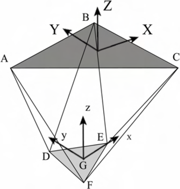
–Graphical representation of the Robocrane
As shown in Fig. 1, in order to study kinematics and dynamics of the Robocrane two frames are employed:
The reference frame (XYZ), with its origin in the center of the fixed support (the upper triangle with vertices A,B, and C) The body frame (xyz), which is similarly attached to the movable platform (the lower triangle with vertices D, E, and F).
In this section, kinematics and dynamics of the robot will be studied by use of two different sets of motion variables; the first set of variables which has been frequently used to study 6 d.o.f cable robots in previous researches and we call it the “conventional set”, and the second set which can be called the “new set”.
Since the robot has six degrees of freedom, at least six independent motion variables are needed. Conventionally, the following set of variables is used in the analysis of 6 d.o.f cable robots;

Where, x, y, and z are the Cartesian coordinate of center of mass of the moving platform and α, β, and γ are Euler angles.
Now, using Newton-Euler equations we have:

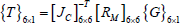
Where, m and [I] are mass and moment of inertia matrix of the moving platform, respectively. The vector in left side represents external forces and moments exerted to the robot. Equation (2) can be written in the following form;

Here, [MC] is the inertia matrix, [RM] is the modified transformation matrix, [JC] is the conventional Jacobian matrix, {C} is the vector of velocity terms, {τ} is the vector of winch torques, {G} is the gravity vector, {L} is the external load vector and r0 is radius of drum of the winches. It should be noted since the cables are only capable of pulling, each of the elements of {τ} must be non-negative, otherwise it is put zero in the equations of motion.
In equation (3), [RM] is;

Where, [R]3×3 is the rotation matrix between the two introduced frames.
As stated, in equation (3), [JC] is the conventional Jacobian matrix which relates time rate of change in lengths of the cables to the velocity and angular velocity of the moving platform as follows;
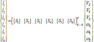
Where;

In equations (6), vectors r and u are the position and unit vectors (in the directions of the specified points), respectively.
Here, we introduce {XN} as follows;

Unlike the conventional set, the new set consists of nine variables. As it is observed, the elements of {XN} are the Cartesian coordinates of vertices of the moving platform written in the reference frame. Here, Lagrange method is used to derive the equations of motion. Therefore, we can consider the variables in question as generalized coordinates. It is clear that these generalized coordinates are not independent. In other words, since the robot has six degrees of freedom, three constraint equations are also needed. These equations are;

Where, a is half of the side of the lower triangle. Equations (8) imply that the distances between vertices of the lower triangle remain constant.
In derivation of the kinetic energy in terms of the discussed generalized coordinates, it is convenient to use point masses instead of distributed mass. Otherwise, we encounter complicated terms in the rotational part of the kinetic energy.
The moments and products of inertia of the moving platform are;

It should be noted that the thickness of the lower triangle in calculation of the moments of inertia is ignored.
As it is shown in Fig. 2, four point masses are positioned in the moving platform; three identical masses (m2) at the vertices and a single point mass (m1) at the center of mass of the lower triangle. Now, we can determine m1 and m2 so that the masses and mass moments of inertia of these systems are identical;

Equations (10) lead to;


– The moving platform with the point masses
It should be noted that it is not necessary to check equality of the other moments of inertia (Iyy and Izz) because these equations and the second equation in equations (10) are dependent. It is clear that the products of inertia of these systems (Ixy, Izx, and Izy) are identical regardless of values of the unknowns, as a result of this arrangement of the point masses.
Now, the kinetic and potential energies of the robot are easily expressed in terms of the generalized coordinates. Then, the equations of motion can be derived;
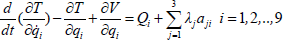
It leads to;

Here, [MN] is the new inertia matrix;

In equation (13), we also have;


Where, [a] is the Jacobian constraint matrix, {λ} is Lagrange multiplier vector.
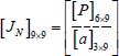
In addition, [P] in equation (13) is the matrix which relates the vertex velocities to the joint velocities as follows;

If we write equation (13) in the following form;

Then, we can define the new Jacobian matrix as;
Therefore we have;

Or;

Where, elements of the new Jacobian matrix are components of unit vectors in specified directions. The previous equation completely expresses all of the kinematical relations of the system. Because of using Lagrange multipliers, the three last elements in the left side of equation (22) are zero. In other words, it is like that three additional degrees of freedom are given to the robot by replacing the sides of the lower triangle with hydraulic pistons, and then they are locked (i.e. i7 = i8 = i9 = 0).
In equation (19), {Q} is the generalized force vector which is obtained by calculation of virtual work done by external loads (except the gravity force). In the case where we also have external moments, Because of difficulty in expressing virtual rotation of the moving platform in terms of the generalized coordinates, we replaced each of three external moment components (in xyz frame) with forces in point masses so that the sum of them vanishes but they produce the moment in the corresponding direction (see Fig. 3).

–Replacement of the external moments by forces
Now, {Q} can be obtained from the following equation;

Where, {L} is the external load vector;

And, [W] is the matrix with rows which specify contribution of the external loads to each generalized force as follows;

Where, Rij's (elements of the rotation matrix) can be easily obtained in terms of the new variables without any angular parameter regarding the fact that the columns of [R] are the basic unit vectors of the body frame (i, j, and k), written in the reference frame.
Definition of Jacobian Matrix Using the Concept of Constraint
In definition of the new Jacobian matrix, we inserted the velocity constraints in equation (22) to achieve a complete expression of the system kinematics. Although the robot has six degrees of freedom, we considered it as a 9 d.o.f system with three inactive degrees of freedom. In other words, the added degrees of freedom are three “virtual degrees of freedom” which appeared in kinematical relations as a result of using constraints. This new approach employed to define Jacobian matrix has not been used before and distinguishes this research from previous studies.
Efficiency in Workspace Determination
The workspace of a cable robot is characterized by the set of points where the center of the moving platform can be positioned while all cables are in tension and their lengths are less than a maximum limit. Therefore, in order to determine the workspace of cable robots, the equations of motion are also needed. Because of complexity in determining the workspace of cable robots by analytical methods, numerical methods are extensively used by researchers. The main disadvantage of numerical methods is their exhaustive and time-consuming search in the entire taskspace.
Checking the cable tensions in each point by use of equations of motion is an important part of the exhaustive search. Here, either the conventional or the new equations of motion can be used;
Equation (26) is derived from the conventional equations of motion and yields the cable tensions for the static case when the gravity is the only external force exerted to the robot. However, if we use the new form of equations of motion, we have;

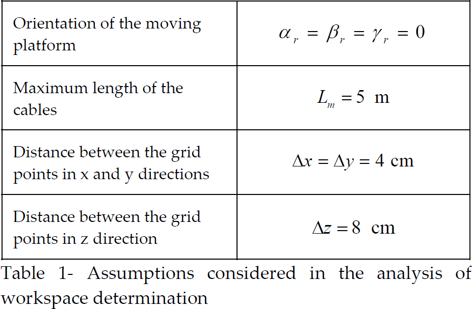
For comparison, two programs were created in MATLAB to determine the static constant-orientation workspace of the Robocrane for a special orientation by both methods. To do that, a three dimensional grid of points was considered and the condition of falling into workspace in each point was investigated. Assumptions of the analysis are specified in Table 1.
Assumptions considered in the analysis of workspace determination
The workspaces obtained by these programs are identical as shown in Fig. 4.
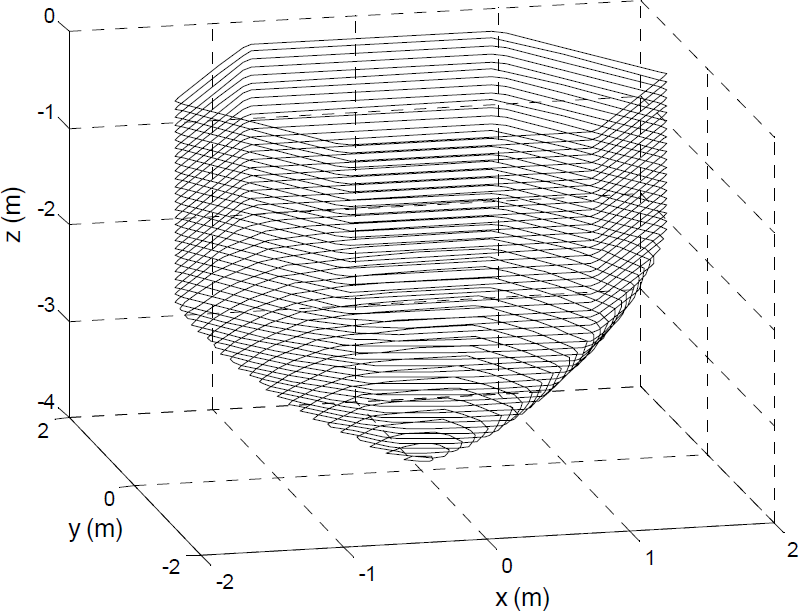
Workspace of the robot (for 4aL=β=γ=0 orientation)
The difference between these programs is in the time it takes to obtain the workspace as indicated in Table 2;
Comparison between efficiency of the two methods in workspace determination

As it is observed, the computation time in the new method is about 36% of the computation time in the conventional one. Such computational efficiency is more considerable when workspaces for several orientations (e.g. for workspace optimization) are to be obtained.
Here, we assumed that it is desired to obtain the required motor torques for a movement of the lower triangle in a special path within a specified time (tf). Therefore, two programs were created in MATLAB and then, the motor torques (as functions of time) and the required time for computation in each program were obtained and compared. Assumptions of the analysis are specified in Table 3.
Assumptions considered in the analysis of solving equations of motion

Assumptions considered in the analysis of solving equations of motion
According to the assumptions in Table 3, each motion variable follows a fifth order polynomial from its initial value to final value. The velocities and accelerations in the start and end points of the path are zero. The path unknowns (vectors ai‘s) in each program are determined so that the initial and final conditions are satisfied. In the program written for the new method, the initial and final position vectors are obtained from the corresponding position vectors specified in Table 3.
The winch torques obtained by these programs are identical as shown in Fig. 5.
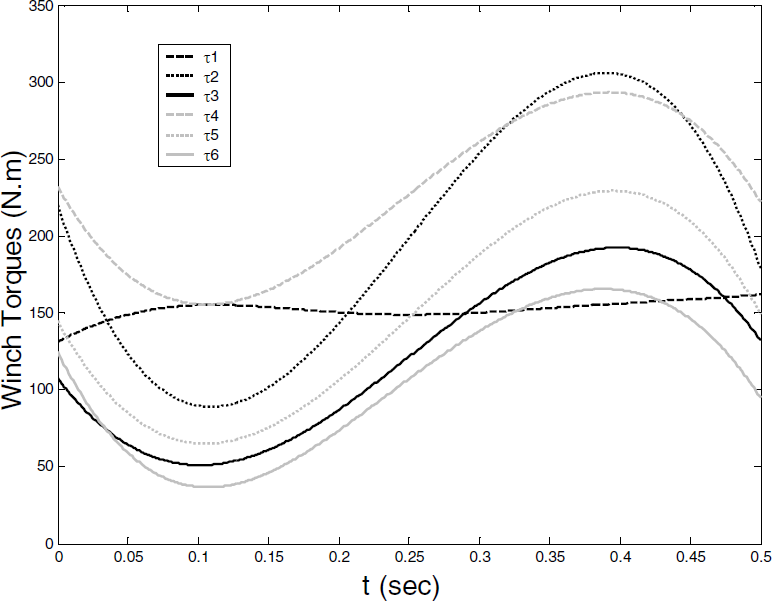
–The winch torques as functions of time
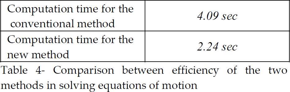
Comparison between these programs reveals that the computation time in the new method is about 54% of that in the conventional one (see Table 4) and the difference can be more considerable when the movement time (tf) is longer. Absence of trigonometric functions, and simple algebraic terms in equations derived by the new method, lead to such computational efficiency in comparison with the conventional method. This reduction of computation time is valuable for purposes like real-time control of cable robots.
Comparison between efficiency of the two methods in solving equations of motion
In this study, NIST Robocrane as a well-known 6 d.o.f cable robot was considered and the Cartesian coordinates of vertices of its moving platform were used as new motion variables to obtain equations of motion. Then, the Jacobian matrix associated with these new variables was introduced. Because of using Lagrange multipliers, three virtual degrees of freedom appeared in this matrix. The approach used to define the new Jacobian matrix distinguishes it from the conventional one. Finally, using programs created in MATLAB, it was demonstrated that the new method is computationally more efficient than the conventional one in workspace determination as well as in solving equations of motion.