Sage Journals: Discover world-class research

Abstract

In this paper, the methods of a snake-like robot climbing on high voltage transmission lines are presented. The three typical locomotion modes of a snake-like robot, that is, rectilinear locomotion with a Zshaped clamping mechanism, obstacle navigation locomotion with a head part clamping mechanism and winding obstacle navigation locomotion, are discussed. The motion mechanism of the snake-like robot's head part clamping obstacle navigation is studied and the kinematics model coupled with the robot and the line environment under this mode is introduced. The position tracking algorithm and the improved algorithm of robot's clamping obstacle navigation are also proposed. Finally, the simulation experiment verifies that the improved position tracking algorithm can improve the robot's motion performance and is feasible in the robot's clamping obstacle navigation.

Keywords

Snake-Like Robot High Voltage Transmission Lines Clamping Obstacle Navigation Climbing

1. Introduction

Overhead high voltage transmission lines are an important medium in electric power transmission and its safe and stable operation directly affects the quality of the power supply in the electric power system. With the enlargement of the capacity of electric power systems, the distribution of transmission lines becomes wider and wider, and most overhead transmission lines are in areas far from towns, with complex terrain and harsh environment. As electric cables, as well as pole and tower accessories, are exposed outside for long periods of time and influenced by continuous mechanical tension, ice hazards, shakes, defilements and material aging, high voltage cables are prone to problems such as broken strands, abrasion and corrosion, which causes hidden trouble in the safety of the electric power supply. An automatic inspection robot for overhead high voltage transmission lines can realize the automatic inspection of transmission lines without any manual intervention and is an effective measure to stop hidden trouble in transmission lines. Moreover, it is highly valued by the power industry and government departments in various countries due to its relatively low labour strength, high efficiency and low cost for inspections.

In recent years, research institutions at home and abroad have shown a great interest in high voltage inspection robots [1 –9]. The prominent research institutions in this field include IREQ (“Institut de recherche en électricité du Québec”, Quebec Electricity Research Institute) in Canada, Kyushu and Chubu Electric Power in Japan, Japan University of Political Science and Law, North Carolina State University in America, KERI (Korea Electrotechnology Research Institute) in Korea, etc. [2, 7, 8, 10 –18]. In addition, research institutions in China, such as Shenyang Institute of Automation of the Chinese Academy of Sciences, CASIA (The Institute of Automation of the Chinese Academy of Sciences), Wuhan University, Shandong University, Shandong University of Science and Technology, Tianjin University, Shanghai University, etc. have carried out important research on inspection robots for single or multiple split live wires and ground wires of different voltage classes [2 –4, 19 –24]. Some prototypes can automatically stride across various typical obstacles, such as counterweights, strain clamps, suspension clamps, jumper wires, etc. Sawada et al. have studied a kind of mobile robot [15] that can inspect ground wires and realize obstacle navigation through guide rails. However, this kind of robot has poor adaptability. Sato, a company in Japan, has produced a kind of line-tracking robot [6] that can detect faults in transmission lines and walk on the ground using remote controls, but cannot realize obstacle navigation. Serge Montambault et al., researchers at IREQ, have developed a kind of remote control robot named HQ LineROver [11] that can achieve the functions of de-icing, inspection and maintenance of power cables, but does not have the ability to cross obstacles and can only work between two pylons. Jaka Katrasnik, a researcher at the University of Ljubljana in Slovenia, has proposed a kind of robot that can climb as well as fly [13]. Nicolas Pouliot has also proposed a kind of line-tracking robot based on LineScout technology [11], which has two parallel arms, one for rolling and another for moving on cables [12]. Paulo Debenset has designed a kind of line-tracking robot that can climb on four-splitting leads [25].

Snake-like robots are a new research interest in the field of robotics and their application includes areas of medical treatment, fault localization, search and rescue and outer space exploration [26 –28] due to its special structural form and flexible control methods. However, the research into snake-like robots climbing high voltage cables is almost non-existent. The idea that snake-like robots could be used to climb high voltage transmission lines was first proposed by Hideo Nakamura et al. at the Japan University of Political Science and Law. They put forward a kind of inspection robot with an electric train and feed cables [19], which is, however, unsuitable for crossing obstacles with larger diameters and intervals. By utilizing the features of the high redundancy of its degrees of freedom (DOF) and its flexible structure and in order to suit the complex and changing line environment, a brand new technical scheme of snake-like robots for use on high voltage lines is proposed in this paper, which expands the application range of snake-like robots.

At present, snake-like robots can be mainly classified into three types: ground creeping snake-like robots, underwater swimming snake-like robots and climbing snake-like robots. The climbing robots can also be divided into inner-climbing and outer-climbing. The climbing snake-like robots that twist on high voltage lines may be regarded as a kind of outer-climbing snake-like robot. There are essential differences between outer-climbing snake-like robots and ordinary ground creeping snakelike robots. The ground creeping snake-like robot realizes its movement by using the friction between the “snake body” arising from its own motion process and the ground to generate propulsion, while the outer-climbing snake-like robot belongs to a three-dimensional space motion mechanism. Its normal pressure is generated by a winding force and the winding force and the contact frictional force need to be controlled simultaneously in the process of climbing. The process of winding and climbing can be considered as the multi-body coupling of the robot, as well as the results of the multi-body dynamic coupling of the contact coupling between the “snake body” and the surface of conductors.

There are relatively few studies on outer-climbing snakelike robots. The representative research institution in this field is Carnegie Mellon University in America, which has designed a robot named Modsnake [33]. It can creep on smooth and vertical glass pipes, which it achieves by using the movements of winding and rolling. Sun Hong, a researcher at Shanghai Jiao Tong University in China, has proposed a kind of outer-climbing snake-like robot based on P-R modules [34]. It adopts an inchworm locomotion gait, the climbing movements are accomplished through the delivery of locomotion wave from its tail to its head and the climbing track is always based on isometric spirals. The two locomotion modes can both result in climbing by a snake-like robot on high voltage transmission cables, but their movement efficiency is relatively low. In order to increase the inspection speed of robots on electric cables, a climbing method that combines Z-shaped clamping climbing with spiral and winding climbing over obstacles is presented in this paper. This method of climbing can improve the speed of inspections in a straight line. This scheme has many advantages compared with the present traditional power line robot, such as better adaptability to the power line and lighter and lower energy consumption.

This paper arranges its content as follows. The second section introduces the line environment for the work of a snake-like robot and then the unit structure and the walking and obstacle navigation methods of the snake-like robot are presented. The third section introduces the mechanism of the snake-like robot's head clamping obstacle navigation, including the kinematics and kinetics model coupled with the robot and the line environment. The fourth section describes the position tracking algorithm and the improved algorithm related to the robot's clamping obstacle navigation and the fifth section makes a simulation analysis of the kinematics and kinetics for the methods proposed in the paper. Finally, the research work is summarized and future improvements are outlined.

2. Background information

2.1 The environment of high voltage transmission lines

The structure of high voltage transmission lines consists of a transmission line tower, a live wire and a ground wire. The live wire is the main medium of power transmission and is usually made of ACSR (aluminium cable steel reinforced). The live wire is hung between transmission line towers in the form of catenaries and the suspending supports and insulation requirements for high voltage transmission lines are guaranteed through hardware fittings and insulators between the transmission line towers and the live wires. The high voltage transmission line itself has certain flexibility and slight vibrations will occur under the periodic wind load.

There are three common types of hardware fittings in single split live wires: counterweight, suspension clamp and strain clamp, as shown in Fig. 1. Although the hardware fittings used in high voltage transmission lines have strict procedures for design and manufacture, their structure is usually complicated, their installation size has some degree of randomness on high voltage transmission lines and they will be corroded, deformed and loosened for years under the action of physics and chemistry in nature. All these elements make the environmental model of high voltage transmission lines complex, thus it is difficult to describe the complex line environmental structure using a single mathematical model. The line-tracking robot must have the ability to cross obstacles, so that they can run through the whole line intervals due to the existence of these hardware fittings.

Figure 1.

Three typical kinds of obstacle at high voltage transmission lines

The common features of the three typical kinds of obstacle can be summarized: 1. the structure of the three obstacles can be considered as consisting of two rectilinear wires (jumper wires can be partially equivalent to rectilinear wires), 2. the plane, which is made up of high voltage transmission lines and hardware fittings, can be approximated to be a vertical plane and the plane that is made up of the two wires may deviate from the vertical plane under the influence of natural wind, the diversity of geographical environmental structures, etc.

Therefore, a simplified model of a transmission line can be obtained, as shown in Fig. 2. This model consists of two rectilinear wires (equivalent to slender cylinders) and its inertial coordinate system of {O} can be established, where the x-axis is the extending direction of Line 1 to Line 2, the z-axis is perpendicular to the x-axis and parallels the vertical plane with an upward direction as its positive direction. Supposing Point A is a point in the x-axis, Plane OAB is a vertical plane, Plane OAC is a plane that consists of Line 1 and Line 2, α is the angle between the two planes and β is the angle between Line 1 and Line 2.

Figure 2.

The simplified model of high voltage transmission line

2.2 The unit structure of a snake-like robot

The unit structure of the snake-like robot's joints proposed in this paper is shown in Fig. 3. It is composed of two space orthogonal rotation mechanisms and a swing mechanism of road wheels. The two orthogonal rotation mechanisms are driven by two steering gears and realize their assembly and connection through steering gear connectors. Rudder connectors are fixed on the connection plate of one of the steering gears. The snake-like robot can be assembled through alternate combination with the steering gear connectors and the rudder connectors. The road wheels are assembled at the side of rudder connectors in each unit and they are driven by electric motors to provide driving torques for the robot when it is walking on high voltage transmission lines.

Figure 3.

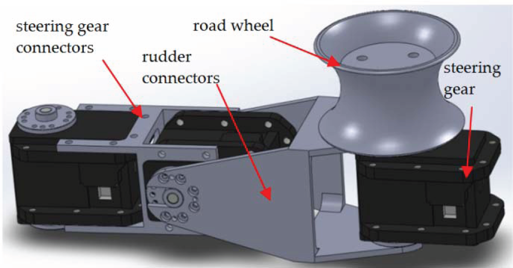
A three dimensional structural diagram of the robot's unit

A two dimensional assembly diagram of the robot's unit is shown in Fig. 4. There are some critical structure sizes that can affect the obstacle-navigation control of the robot in Fig. 4, including: l₁- the centre distance of the rotation axis of the two steering gears connected by steering gear connectors, l₂- the centre distance of the rotation axis of the two steering gears connected by rudder connectors, W₁- the distance from the symmetrical centreline of the robot's unit to the symmetrical plane of the road wheels in their walking direction, D₁- the minimum external diameter of the road wheels and H₁- the distance from the symmetrical plane of the road wheels to the plane of the outer edge of the road wheels. These size parameters are also critical to establishing the kinematical equation of the robot.

Figure 4.

The assembly diagram of the robot's unit

2.3 The rectilinear locomotion of a snake-like robot

The robot uses a locomotive mode, which is shown in Fig. 5, on the straight-line segment of transmission lines. The robot is unfolded in the shape of a “Z”. The high voltage transmission line is clamped by the robot in the middle position between the top and bottom road wheels and the clamping force on the high voltage transmission line can be adjusted through the adjustment of the robot's pitching joint torques. In order to balance the roll torques caused by the weight of the robot, some joints of the robot break away from the wires to adjust the centre of gravity. Moving the whole robot forward or backward can be achieved through the control of each road wheel's motor speed. The rotating speed of each electric motor in contact with the lines must be given in accordance with the following formulae, so as to satisfy the coordinated and consistent forward movement of robot.

Figure 5.

The rectilinear locomotion of a snake-like robot

{\begin{matrix} ω_{i} = \frac{v}{R} & i = 1, 3, 5 \dots 2 n + 1 \\ ω_{i} = - \frac{v}{R} & i =2, 4, 6 \dots 2 n \end{matrix}

(1)

where v is the given forward speed of robot, R is the radius of the road wheels, n is an integer and i is the number of robot units (as shown in Fig. 5).

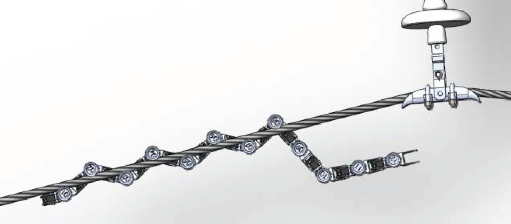
2.4 The method of a snake-like robot's head part clamping obstacle navigation

A sketch map of the robot's head part clamping obstacle navigation is shown in Fig. 6.

Figure 6.

The state of head part clamping obstacle navigation

The robot can be divided into three parts according to their functions: the first part is the head clamping part, which is used to grasp Line 2 at the rear of the hardware fittings, the second part is the tail clamping part, which is used to grasp Line 1 at the front of the hardware fittings, the remaining part is the middle adjustment unit, which is used to adjust the position and posture of the head clamping part relative to Line 2. The tail clamping part and head clamping part in the figure are both made up of four units and, if necessary, the actual quantity can be adjusted properly. The detailed process of obstacle navigation is as follows:

The robot moves and stops at the front of obstacles and the joints in its head and middle parts gradually deviate from the lines. Only the four units of the tail clamping part are retained to grasp the lines. The robot is then ready to cross obstacles.

The road wheels of the tail clamping part are controlled to move forward until they are close to the obstacles (suspension clamps).

The four joints at the head part are adjusted into a Z-shaped clamping pose at the proper position of the head clamping part, close to the other part of the lines.

The head clamping part is moved gradually closer to Line 2 and when the line is in a position that is suitable to grasp, the head clamping part grasps the line.

The tail clamp holder is loosened to make the tail of the robot gradually deviate from the line, the whole robot moves forward along Line 2 to make it cross the obstacles and the robot is adjusted to a walking state to make it move on.

The key technology of the head part clamping obstacle navigation is establishing a proper mathematical model in kinematics and kinetics, coupled with the robot and the line environment. The rotation angle of the joints in the middle adjustment unit is controlled based on the model so as to achieve the purpose of adjusting the position and posture of the head clamping part. The research in this paper mainly focuses on this method of obstacle navigation.

2.5 The method of a snake-like robot's winding obstacle navigation

Winding obstacle navigation is a method of obstacle navigation that takes full advantage of the structure of the snake-like robot. The implementation method is as follows. First, when the robot approaches an obstacle, make the joint units at its head and middle parts deviate from the lines as much as possible. Second, wrap the obstacle with a winding method. Third, move the robot slowly along the obstacle by virtue of its own inchworm locomotion until the whole robot breaks away from the obstacle. Finally, adjust the robot in a walking state. Further research on this method of obstacle navigation will be carried out in the follow-up work.

3. The mathematical model of head part clamping obstacle navigation by a snake-like robot

3.1 The kinematics model of snake-like robot

The mathematical model of a snake-like robot is shown in Fig. 8, supposing the initial pose of the robot is arranged along Line 1 in a straight line.

Figure 7.

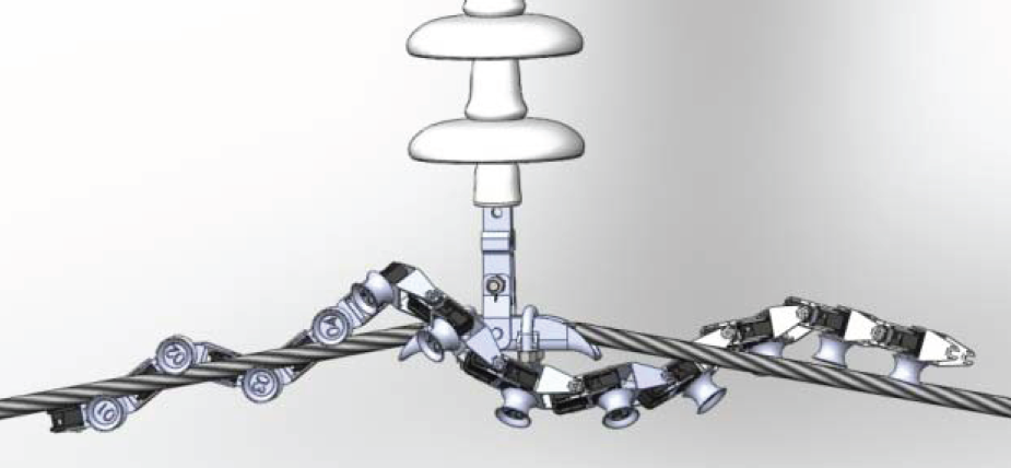
The state of robot's winding obstacle navigation

Figure 8.

The mathematical model of the snake-like robot and its environmental structure

The pitching joint located at the road wheel of the last contact wire of the tail clamping part is considered to be Joint 1 and the other joints in the middle adjustment unit are numbered in order according to their distance from Joint 1. For the sake of convenience, several types of coordinate system are established as follows:

The base coordinate system of robot - {B}: the origin of a coordinate is the central position of Joint 1, the x-axis stays the same as the symmetrical centreline of the initial position of the robot modular structures and the positive direction of the x-axis is from the tail part to the head part of the robot. The y-axis is the axis of Joint 1 with a direction from the road wheel to the steering gear.

The tool coordinate system of robot - {T} is fixed at Link 2n-1 (n is a positive integer) of the robot and the coordinate system of {T} in the figure is set up at Joint 7. The origin of the coordinate is the geometric centre of the road wheel and the positive direction of the x-axis points to the head part of the robot. The y-axis is the rotary axis of the road wheel, which is located at the module of the coordinate system and the positive direction of the y-axis is from the road wheel to the steering gear.

The kinematical equations of a snake-like robot are set up according to the amended D-H method. The equations overlook the rotary motion of the road wheel and only consider the pitching and deflection motion of the middle joints of the robot. The coordinate system of the joints is displayed in Fig. 8 and the transformation matrix of the adjacent links is as follows:

{}_{1}^{B}T = R_{X} (- 90 °) R_{Z} (q_{1})

(2)

{}_{2}^{1}T = R_{X} (90 °) D_{X} (l_{1}) R_{Z} (q_{2})

(3)

{}_{3}^{2}T = R_{X} (- 90 °) D_{X} (l_{2}) R_{Z} (q_{3})

(4)

{}_{i}^{i - 1}T = {\begin{matrix} R_{X} (90 °) D_{X} (l_{1}) R_{Z} (q_{i}) & i = 2 n \\ R_{X} (- 90 °) D_{X} (l_{2}) R_{Z} (q_{i}) & i = 2 n - 1 \end{matrix}

(5)

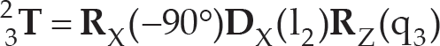
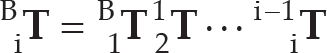
where q_i is the rotation angle of Joint i, ^i–1_iT is the transformation of Link i versus Link i-1 and n is an integer greater than one, so the transformation matrix of Link i relative to {B} (the base coordinate system of robot) can be expressed as:

{}_{i}^{B}T = {}_{1}^{B}T {}_{2}^{1}T \cdot \cdot \cdot {}_{i}^{i - 1}T

(6)

The transformation matrix of {T} (the tool coordinate system of robot) versus {B} (the base coordinate system of robot) is established. Supposing the origin of {T} is the centre of the nth road wheel, the Link i fixed with {T} will be Link 2n-1. As:

{}_{T}^{i}T = D_{Z} (- w 1) R_{X} (90 °)

(7)

Therefore, it can be known that:

{}_{T}^{B}T = {}_{i}^{B}T {}_{T}^{i}T = {}_{i}^{B}T \times D_{Z} (- w 1) R_{X} (90 °)

(8)

3.2 The kinematic coupling model of the robot and the line

The robot only relies on its road wheels being in contact with the wires in the process of obstacle navigation with a kind of tail clamping mechanism, so the relationship between the road wheels and high voltage transmission lines is contact coupling. Although high voltage transmission lines possess certain flexibility, they have little flexible deformation even under conditions of full tension, so they can be taken as rigid structures. The robot body consists of many rigid structures, so it can also be considered as multiple rigid structures. Therefore, the coupling model of the robot and the line environment can be simplified as the coupling model of multiple rigid structures. As the motion types of the robot's tail clamping part relative to high voltage transmission lines are mainly the movement along the direction of the transmission lines and the rotation along the direction of the shaft axis of the transmission lines, the complex contact coupling between the road wheels and the wires can be expressed as the equivalent combined model of a sliding pair and a revolute pair.

For convenience, the general mathematic model of the robot and line environment, as well as the following types of coordinate system, is established:

The work coordinate system of robot - {S} is fixed at Line 2 and the z-axis coincides with the rotation centreline of Line 2. The y-axis is perpendicular to the plane consisting of the centres of Line 1 and Line 2.

The target coordinate system of robot - {G} is established for the head part of the robot being close to Line 2 with the right pose; if the robot wants to realize the grasp of Line 2 with the correct pose, the tool coordinate system of {T} must coincide with the target coordinate system of {G}.

The inertial coordinate system of {O} remains stationary with the earth and is set up mainly for the establishment of the kinetic model. The origin of a coordinate is the crossing point of the centrelines of Line 1 and Line 2. The z-axis is vertically up and the x-axis is consistent with the centreline of Line 1 with the positive direction of Line 1 pointing to Line 2.

The following transformation needs to be carried out in the conversion of {B} to {S}:

{}_{S}^{B}T_{G} = {}_{1}^{B}T_{G} {}_{2}^{1}T_{G} {}_{3}^{2}T_{G} {}_{S}^{3}T_{G}

(9)

where the subscript of G refers to the coordinate transformation of the environment and is used to distinguish it from the coordinate transformation of the robot.

{}_{1}^{B}T_{G} = D_{Y} (- w 1) D_{Z} (- \frac{D 1 + D 2}{2}) R_{Y} (90 °) R_{Z} (g q_{1})

(10)

{}_{2}^{1}T_{G} = D_{Z} (g q_{2})

(11)

{}_{3}^{2}T_{G} = R_{X} (- 90 °) R_{Z} (g q_{3})

(12)

{}_{S}^{3}T_{G} = R_{X} (90 °)

(13)

where gq¹ is the upsetting angle of the tail clamping part relative to the initial position, gq² is the distance from the central point of the rightmost road wheel at the tail clamping part to the origin of the work coordinate system along with the direction of the axis of Line 1 and gq³ is the deflection angle of the target Line 2 relative to the initial Line 1.

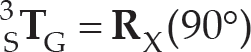
The following is a series of transformations, which need to be carried out in the conversion of {B} to {G}:

{}_{G}^{B}T_{G} = {}_{1}^{B}T_{G} {}_{2}^{1}T_{G} \dots {}_{7}^{6}T_{G} {}_{G}^{7}T_{G}

(14)

where:

{}_{4}^{3}T_{G} = R_{X} (90 °) D_{Z} (g q_{4})

(15)

{}_{5}^{4}T_{G} = R_{Z} (g q_{5})

(16)

{}_{6}^{5}T_{G} = D_{Z} (g q_{6})

(17)

{}_{7}^{6}T_{G} = R_{Y} (- 90 °) D_{Y} (g q_{7})

(18)

where ⁷_GT_G is the unit matrix of order four, gq⁴ is the distance from the origin of the work coordinate system to the origin of the target coordinate system along the direction of the axis of Line 2 and represents the displacement distance of the target road wheel along the direction of Line 2, gq⁵ is the flip angle along the axis of Line 2 and represents the deflection angle of the target road wheel relative to the axis of Line 2, gq⁶ is the translational distance along the direction of X_g⁶ and represents the normal distance of the road wheel deviating from the circumscribed circle of lines and gq⁷ is the translational distance along the direction of Y_g⁷ and represents the tangent distance of the road wheel deviating from the circumscribed circle of lines.

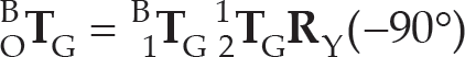
In addition, the coordinate transformation of {B} to {O} can be obtained as follows:

{}_{O}^{B}T_{G} = {}_{1}^{B}T_{G} {}_{2}^{1}T_{G} R_{Y} (- 90 °)

(19)

The following can be known according to the operation rules of coordinate transformation:

{}_{T}^{S}T_{G} = {}_{B}^{S}T_{G} {}_{T}^{B}T_{G}

(20)

{}_{G}^{S}T_{G} = {}_{B}^{S}T_{G} {}_{G}^{B}T_{G}

(21)

{}_{B}^{S}T_{G} = [\begin{matrix} {}_{S}^{B}R_{G}^{T} & - {}_{S}^{B}R_{G}^{T} {}^{B}P_{S O} \\ 0 & 1 \end{matrix}]

(22)

where ${}_{S}^{B}R_{G}$ refers to the rotation transformation of ${}_{S}^{B}T_{G}$ , ${}^{B}P_{S O}$ refers to the translation transformation of ${}_{S}^{B}T_{G}$ and the superscript T refers to the transpose of this matrix.

When using the tool coordinate system as a reference coordinate system, the Jacobi transformation matrix of the robot can be obtained by the following formulae:

{}^{T}J_{i} = [\begin{matrix} {(P \times n)}_{z} \\ {(P \times o)}_{z} \\ {(P \times a)}_{z} \\ n_{z} \\ o_{z} \\ a_{z} \end{matrix}]

(23)

where ${}^{T}J_{i}$ is the Column i of the Jacobi matrix.

When using the work coordinate system as a reference coordinate system, the Jacobi transformation matrix of robot can be obtained by the following formulae:

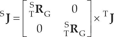
{}^{S}J = [\begin{matrix} {}_{T}^{S}R_{G} & 0 \\ 0 & {}_{T}^{S}R_{G} \end{matrix}] \times {}^{T}J

(24)

where ${}_{T}^{S}R_{G}$ is the rotation transformation part of the ${}_{T}^{S}T_{G}$ matrix.

Through the above transformation, the transformation matrix of the robot relative to the coordinate system of {S} can be obtained.

4. The control method of clamping obstacle navigation of snake-like robot

The snake-like robot can realize the process of obstacle navigation according to the control system framework in Fig. 9. The control strategy modules of obstacle navigation have the functions as follows: to plan the path of the robot in the whole process of obstacle navigation, to deal with the distance of gq¹ and the upsetting angle of gq² outputting from the kinetic model and to correct the path of robot in the process of obstacle navigation timely.

Figure 9.

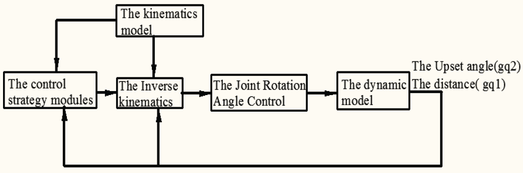
A block diagram for the control of a traditional robot

The inverse kinematics solution proposed according to the strategies of obstacle navigation in the kinematics model is a kind of inverse computation in kinematics for target location and can calculate the rotation angle of each joint in real-time. The process of the inverse kinematics solution also needs to receive the key parameters of gq¹ and gq² outputting from the kinetic model in real time. If the accurate positioning of a six-DOF space of the tool coordinate system is realized, as for six- DOF robots, the definite unique solution can be calculated. However, the snake-like robot proposed in this paper is a kind of redundant robot with more than six DOF and for this type of robot there are infinite numbers of solutions, so optimization algorithms, including gradient descent, optimal dynamics performance, etc., are needed to find the optimal solution.

Moreover, if the head clamping part of the robot proposed in this paper realizes the grasp of Line 2, the translation and rotation along the direction of Zs in the work coordinate system of {S} have no direct effect on the clamping movement; that is to say, the two DOFs can be unrestricted. Therefore, the robot proposed in this paper only needs four DOFs to realize clamping of the target line. Therefore, if the number of joints in the middle adjustment unit is more than four, it will be considered as a redundant robot. In order to improve the control flexibility and the ability of obstacle avoidance of the robot, more than six joints at the middle adjustment unit are adopted in this paper.

As for the redundant robot with multiple DOF proposed in this paper, the inverse kinematics solution of the robotic equation is the key to obtaining a good motion planning control. At present, there are many scholars who engage in research on methods to solve the inverse kinematics solution for the redundant robot with multiple DOF. Shuuji Kajita, a Japanese scholar, has proposed a kind of numerical method of inverse kinematics for biped robots and its principle is to modify joint angles and recycle them when there are differences between the result of forward kinematics and the target value [29]. Zu Di has put forward a kind of secondary calculation used to solve the inverse kinematics of redundant robots [30]. Masayuki Shimizu has proposed a kind of closed solving method for the inverse kinematics solution based on parameterization methods [31] and Antonelli presents an improved optimization method for the inverse kinematic solution of redundant robots and the maximum speed limit of joints can be taken into account in this method [32]. Musto presents a novel computational algorithm for selecting an optimal inverse kinematic solution in response to a pose specification in a redundant robotic manipulator [33] and Chih-Jer Lin has proposed a kind of inverse kinematic solution based on fuzzy reasoning [34].

Based on Shuuji Kajita and Antonelli G's research, this paper adopts an improved coordinate follow-up control method to solve the problem of inverse kinematics for snake-like robots.

4.1 Standard position tracking algorithm

Supposing the DOF of a snake-like robot is n, q is the joint angle space vector of n × 1 and if X is the operating space vector of m × 1, according to the definition of Jacobi matrix, it can be known that the Jacobi matrix of J(q) is the mapping matrix of robotic joint space velocity vectors to operating space velocity vectors, that is:

\dot{X} = J (q) \dot{q}

(25)

In addition, the Jacobi matrix can also be regarded as the transformation matrix of the differential coefficient movement of joint space to operating space, so the above formula can also be written as follows:

Δ = J (q) d q

(26)

d q = J^{- 1} (q) Δ

(27)

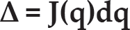
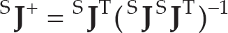
The formula suggests that the deviation of the robotic operating space can find the corresponding deviation of the joint angle space through the inverse operation of the Jacobi matrix. As a great deal of calculation is needed for the whole algorithm, there are unavoidable errors in open loop calculation. Therefore, using the idea of a close loop feedback control for reference, we can compare the given position with the feedback position and improve the position tracking performance of the algorithm through a proportional controller.

The core of the algorithm is shown in the dashed box of Fig. 10, where Xg is the position of the given coordinate system of {G} relative to the coordinate system of {S}, X_fdb is the position of the actual robotic coordinate system of {T} relative to the coordinate system of {S} and ^SΔ is the differential motion vector of the robotic coordinate system of {T} relative to the coordinate system of {G}. The solutions of X_g and X_fdb are obtained respectively from the matrices of ${}_{G}^{S}T$ and ${}_{T}^{S}T$ , and the joint space vector of q and the environment space vector of gq are needed in the calculation process of the two parameters.

Figure 10.

The block diagram for standard position tracking algorithm

^SJ is the Jacobi matrix when using the work coordinate system of {S} as the reference coordinate system and ^SJ⁺ is the inverse of this matrix. As for non-redundant robots, ^SJ⁺ can be directly obtained through the inverse operation of ^SJ in non-singular states, while as for redundant robots, if ^SJ is the full rank, ^SJ⁺ is the pseudo-inverse of ^SJ, that is:

{}^{S}J^{+} = {}^{S}J^{T} {({}^{S}J {}^{S}J^{T})}^{- 1}

(28)

In order to avoid the singular state in the operation process, the dexterity of the robot needs to be monitored in real time. Concretely, this paper uses a conditional index as the index to evaluate the dexterity of the robot. As for redundant robots, m<n, so the robots' dexterity of k(^SJ) can be calculated according to the following formula:

k ({}^{S}J) = | | {}^{S}J | | \cdot | | {}^{S}J^{+} | |

(29)

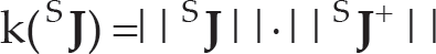
Once the result of k(^SJ) becomes large, it can be concluded that the robots are near singular states. At the moment, the computational process is slow and the error of the calculation is large.

4.2 Improved position tracking algorithm

Although the standard position tracking algorithm mentioned above can find and follow up the target location quickly, it has the following shortcomings:

There is no direct constraint method in the path of a middle course for search targets, which will lead to the path velocity and acceleration calculated through the algorithm exceeding the tolerance limit of the mechanical system.

The target tracking of the robot proposed in this paper under the work coordinate system of {S} may not be constrained for translation and rotation around the z-axis, which helps to improve the tracking and obstacle avoidance of robots for target location. However, using the standard position tracking algorithm, it is difficult to realize the abandonment of tacking for some DOFs.

There is obstacle avoidance involved in the process of obstacle navigation of robots; that is to say, robot manipulators cannot touch transmission lines and hardware fittings. The standard position tracking algorithm needs to adopt complicated optimization algorithms to achieve obstacle avoidance and tracking.

The standard position tracking algorithm cannot solve the above three problems well. Therefore, some simple and effective measures are taken to improve the standard position tracking algorithm in this paper, as shown in Fig. 11. The specific measures include:

Figure 11.

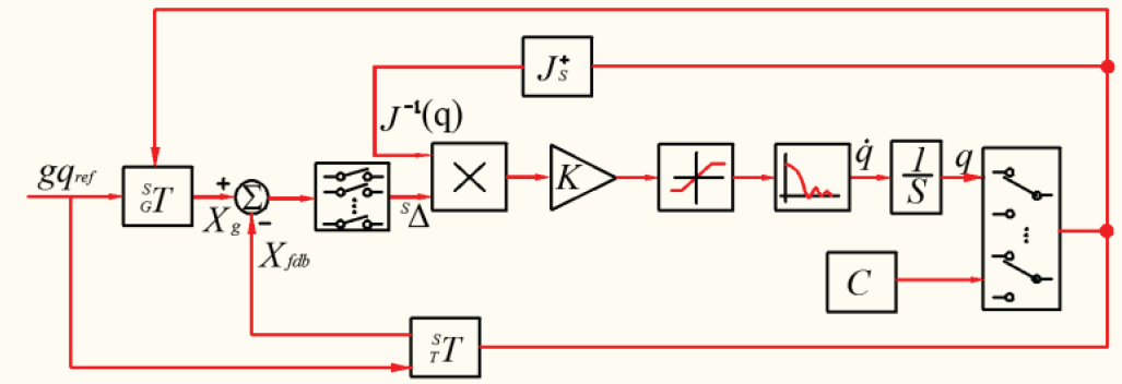
The block diagram for improved position tracking algorithm

Adding the saturation element and low-pass filtering element in the circuit of path generation. The function of the saturation element is to limit the maximum speed of the path and the function of the low-pass filtering element is to limit the acceleration of the joints.

Adding multi-way selective channel before the product of the Jacobi inverse matrix and deviation vectors; that is, open the channel of dz and δz and close the other four channels, which means we will not restrict the dz and δz and could avoid singular status.

Using two-way selectors before the feedback calculation of the outputting joint vector of q. Some selectors choose the outputting joint vector of q, while others choose constants. This will make sure the position and posture of the robot calculated through our algorithm avoids touching high voltage lines and hardware fittings with manual intervention.

4.3 The path planning of the target motion

The path of target trajectory planning is shown in Fig. 12. Supposing the initial state of the robot is in the state of hanging down, the initial angle of Joint 1 is q¹ and the initial angle of the other joints is zero, the origin of the tool coordinate system is Point T. If the robot wants to clamp Line 2, the tool coordinate system of {T} must coincide with the target coordinate system of {G}, where gq⁷ is the centre distance of the target location of Point G to Line 2 and gq⁴ is the distance of Point G to the origin of the inertial coordinate system of {O} along the direction of Z_S.

Figure 12.

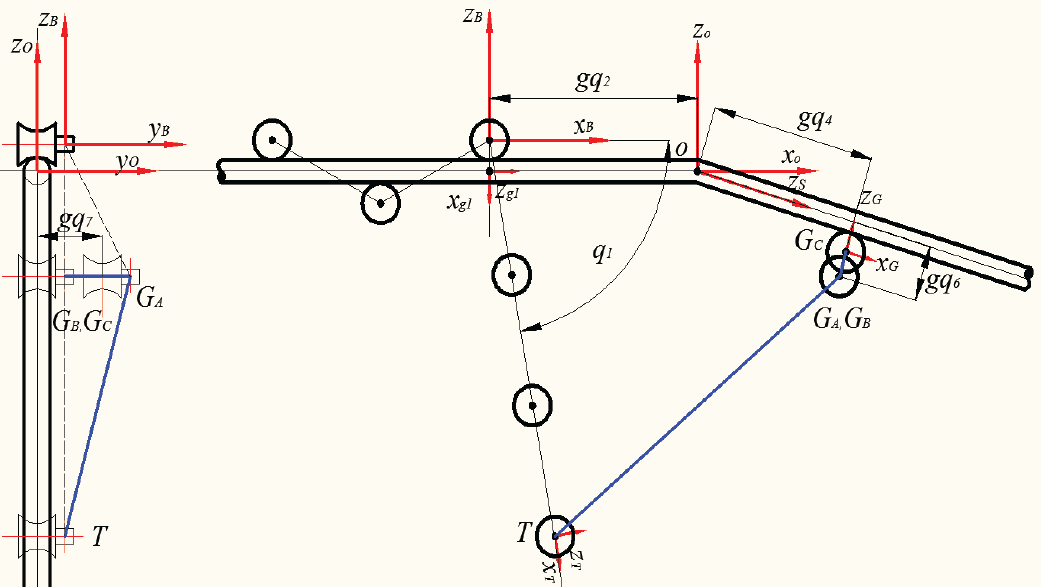
The path of target points

The shortest path of the target trajectory to achieve the robot's grasp movement is the line segment of TG_C, but if this path planning is adopted, the head clamping part of the robot will inevitably interfere with Line 2. Therefore, the middle transition points of Point G_A and Point G_B are set, where Point G_A and Point G_B are on the same horizontal plane and gq⁶ is the distance of Point G_B to the centreline of Line 2. The movement of the robot to grasp Line 2 can be broken down into the following steps:

Under the initial state, the tracking algorithm of the motion path makes the tool coordinate system of robot move in accordance with the track of TG_A and simultaneously makes the head clamping part of robot be in the state of pre-clamping.

Make the target trajectory move in accordance with the path of G_AG_B and make Line 2 be an appropriate clamping pose in the head clamping part of robot.

Make the target trajectory move in accordance with the path of G_BG_C and make the head clamp holder grasp Line 2.

In order to avoid interference in the process of the grasp movement, the following formulae must be satisfied in the first step:

g q_{7} > \frac{D_{1} + D_{2}}{2}

(30)

and

g q_{6} > \frac{D_{2}}{2} + H_{1}

(31)

where Point G_C is the corresponding target point when the road wheel is tangent to the line. It can be known that:

g q_{6} = \frac{D_{2}}{2} + H_{1}

(32)

5. Simulation analysis

5.1 The simulation experiment of the position tracking algorithm

This experiment is to verify the improvement of path generation by the improved algorithm versus the original algorithm. The standard position tracking algorithm, the position tracking algorithm with speed limiters and the position tracking algorithm with speed limiters and filters are used in the experiment to follow up the travelling target trajectory and the waveform data of the following error, the target path velocity and the acceleration are recorded.

A simulation block diagram for position tracking algorithms is shown in Fig. 13, where ref-pos is an input part that receives the environmental model parameters of gq¹∼gq⁷, and Angle_output is an output of the model that outputs the angle information of joints involved in the position tracking of the robot and where the T_SG module is the matrix transformation of {G} versus {T}, the T_ST module is the matrix transformation of {T} versus {S}, the Jacob_S_J module is the pseudo inverse transformation of the Jacobi matrix of the robot in the coordinate system of {S}, the Tr2diff(T2-T1) module is the projection of the difference between two transformation matrices at the space of six-DOF, Route_select1 module is a multichannel gate (only dx, dy, Δx and Δy are gated in this model) and the Route_select2 module is the gating of the outputting joint angles. In the experiment, q1 is identically equal to 80° and the other rotation angles are in an all-pass state. The main purpose of these settings is to avoid the interferential configuration of the robot and the lines.

Figure 13.

A simulation block diagram for position tracking algorithms

The initial robotic joint vector of [q², q³, q⁴, q⁵, q⁶, q⁷] is set to [0, -pi/2, 0, pi/6, 0, 0], the speed limit is 0.1rad/s and the filter transfer function is $\frac{1}{S + 1}$ . The experimental simulation parameters are as follows:

Table 1.

Simulation Condition

Parameters in the simulation model	Value
l1	0.05302m
l2	0.07898m
W1	0.0415m
D1	0.025m
R1	0.018m
gq1	0°
gq2	0.1m
gq3	30°
gq4	0.2m
gq5	0°
gq6	0.035m
gq7	0.05+0.05sin(0.3t-π/2) m

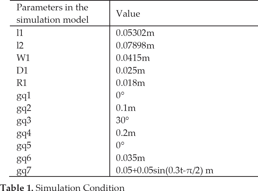
When gq⁷ is in motion in accordance with the change rule given in the table, the target trajectory will have a periodic change. The corresponding tracking effect of the three algorithms is displayed in the figure, where Column 1 is the changing curve of the robotic joint angles involved in the position tracking, Column 2 is the velocity curve of the robotic joint angles, Column 3 is the acceleration curve of the robotic joint angles and Column 4 is the deviation between the target coordinate system and the robotic tool coordinate system.

The waveform in the simulation experiment of the standard position tracking algorithm is shown in Fig. 14a. It can be seen from the figure that the algorithm converges quickly after the operation of the simulation and the following error of several controlled parameters (dx, dy, Δx, Δy) drops rapidly within the range of less than 1×10⁻⁴rad (m), but the maximum velocity reaches 5rad/s and the maximum acceleration reaches 10⁺¹²rad/s². Obviously, such high velocity and acceleration are likely to cause mechanical impact and shock. However, after the use of speed limiters, the velocity is limited within the range of 0.1rad/s, but the peak of acceleration still exists and the maximum acceleration can reach 10⁺¹¹rad/s². The following error of the algorithm with speed limiters is nearly the same as that of the algorithm without speed limiters, as shown in Fig. 14b. After the addition of filters, the acceleration can be limited; it can be seen from Fig. 14c that the acceleration is less than 0.2rad/s², while compared with the first two algorithms, its following error has a little fluctuation, but converges immediately.

Figure 14.

The curve of position tracking performance in the three algorithms

The simulation experiment has verified that the improved algorithm proposed in this paper can effectively make up for the shortcomings of the original algorithm and reduce mechanical impact and shock.

5.2 The simulation experiment for the process of the robot grasping power lines

The purpose of this simulation experiment is to synthetically verify the control strategy proposed in the system. The simulation platform is based on the operating system of a PC with 64bitWin7, 3.4GHz basic frequency and 16G of RAM. The co-simulation method with Adams and Matlab is used in the system for the simulation analysis. The kinetic model is set up based on the platform of Adams and the control system model is set up based on the platform of Matlab. The equivalent of two cylinders is adopted in the environment of high voltage transmission lines in the kinetic model. The four road wheels at the robot's tail retain a compaction state with the high voltage transmission lines under the action of steering gear torques. The rotation of the road wheels is restrained through closed control of the position. As for the joints in the middle adjustment units, the classic PID controlling method is used to control the joint rotation angles. The model dimension parameters of the robot are consistent with physical prototypes. The specific simulation parameters are as follows:

Table 2.
Simulation parameters

Parameters in the simulation model Value

l1 0.05302m

l2 0.07898m

W1 0.0415m

D1 0.025m

R1 0.018m

gq1 0°

gq2 0.1m

gq3 30°

gq4 0.2m

gq5 0°

Weight of steering gear connectors 0.264Kg

Weight of rudder connectors 0.101Kg

Weight of road wheels 0.034Kg

Static friction coefficient between road wheel and line 3.0

Dynamic friction coefficient between road wheel and line 1.0

Clamping torque of at the tail clamping part 3.4Nm

The motion process of the robot is divided into four stages. In the first stage (time duration: 0∼4 seconds) the robot moves gradually closer to Line 2 and the road wheel keeps a safe distance of 5mm from the lines. In the second stage (time duration: 4∼7 seconds) the robot adjusts its pose so that Line 2 is in clamping position in the head clamp holder. In the third stage (time duration: 7∼9 seconds) the robot adjusts its pose so that the road wheels at the tool coordinate are moved gradually closer to the lines and start to grip. In the fourth stage (time duration: 9∼10 seconds) the head of the robot gradually clamps the 2nd power line.

The changing curves of the joint angles (above) and the joint driving torques (below) of the robot in the whole motion process are shown in Fig. 15. The change rule of the joints (except q¹, which remains constant at 80°) is recorded. It can be seen from the changing curve of the joint angles that the change of the joint angles are smooth transitions without any large fluctuations at any motion stage. It can also be seen from the changing curve of the joint torques that the deflection joint torques of the robot (Tq², Tq⁴, Tq⁶)at every motion stage are relatively small, but the pitch moments (Tq³, Tq⁵, Tq⁷) increase gradually at the first motion stage and Tq³>Tq⁵>Tq⁷. The primary reason for the distribution of these moments is that the self weight of the robot decreases progressively at the arm of the force and the acting force of each pitching joint (q³, q⁵, q7).

Figure 15.

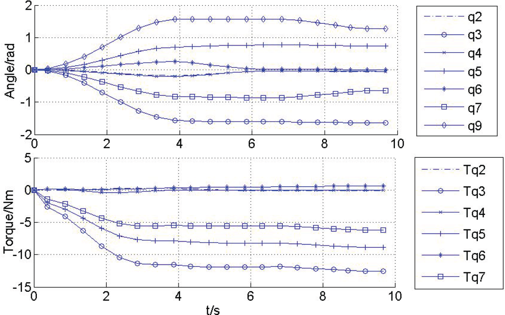
Joint deflection angles and joint torques

The deflection angle moving around Line 1 at the whole motion stages of robot, that is, the environmental model variable of gq¹, is shown in Fig. 16. It can be seen from the curve that the robot has continuous deflection movements around Line 1 at each motion stage, which is caused by unbalanced moments in the process of robotic clamping obstacle navigation. The unbalanced moments are caused by the weight of the robot and the change trend can be reduced by increasing the frictional force between the tail road wheels and the lines.

Figure 16.

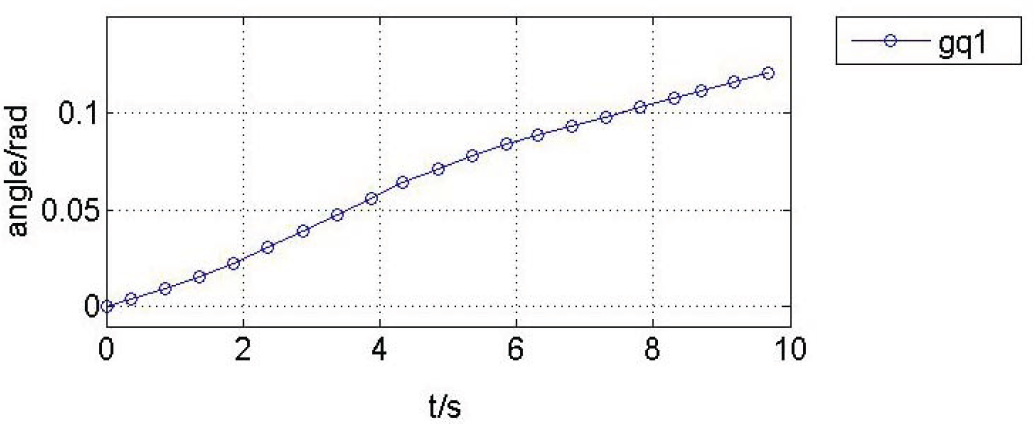
The deflection angle of gq¹

The changing curve of the tracking errors in the whole motion of the robot is shown in Fig. 17. It can be seen that the tracking errors of dx, dy, Δx and Δy tend to be zero, while dz and Δz have some degree of error. This is because the algorithm proposed in this paper only realizes the tracking of the translational distance along the direction of X_S and Y_S and the rotation angle around the direction of X_S and Y_S, but does not take any control measures for the translation and rotation along the direction of Z_S in the coordinate system of {O} in order to improve the flexibility of the robot when grasping power lines and to avoid singularity in the tracking algorithm. Although the robot has a rolling locomotion around Line 1 in the operational process, the locomotion does not have a strong influence on the process of the robot grasping the power lines, which proves that the algorithm proposed in this paper has good adaptivity for the changes of the wire environment.

Figure 17.

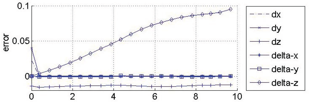
Position tracking errors

In order to evaluate the dexterity of the position tracking algorithm of the robot in the whole operating period, the conditional index in the position tracking algorithm is drawn, as shown in Fig. 18. It can be seen that the conditional index of the robot is within a reasonable range, so there is no singular configuration in the whole operating period.

Figure 18.

The changing curve of the conditional index in the position tracking algorithm of a robot

The animated screenshots of the simulation for the process of the snake-like robot grasping power lines are shown in Fig. 19. Picture a is the initial stage of the simulation, where q¹ is identically equal to 80° and remains immovable in the whole process of the grasp movement and the initial angles of the other joints are all equal to zero. Picture b, Picture c and Picture d are the screenshots of the first stage of the motion process. Picture d is the end of the first stage, where the head part of the robot shows the clamping configuration, the centreline of the clamping configuration parallels Line 2 and the road wheel at the head part clamping configuration keeps a certain safe distance from Line 2. Picture e is the end of the second stage, where Line 2 is in the clamping position of the head part clamping configuration. Picture f is the end of the third stage, where Line 2 is clamped by the head part clamping configuration of robot.

Figure 19.

The simulation for the process of snake-like robot to grasp power lines

6. Conclusion and follow-up work

In this paper, the methods of a snake-like robot climbing at high voltage transmission lines are presented. The motion mechanism of the snake-like robot's clamping obstacle navigation is studied, the simplified models of kinematics and kinetics coupled with the robot and the line environment are put forward and the position tracking algorithm and the improved algorithm for the robot's clamping obstacle navigation are proposed. Through simulation analysis, it can be seen that the method proposed in this paper is effective and feasible in theory. However, the realization of the robot's clamping obstacle navigation is affected by factors of the weight of the snake-like robot, the rotational joints with a large arm of force, etc. Moreover, a suitable method is needed to solve the problem that the pitching joints at the root of the robot (such as q¹, q³, etc.) bear great torque in the process of obstacle navigation. A method of dangling obstacle navigation will be used in the follow-up study. With the help of the action of the robot's inertial force, a method of repeated swinging is adopted to realize the grasp of Line 2 by the head part clamping device. In addition, the method of winding obstacle navigation will also be one of the important components of the follow-up study.

Footnotes

7. Acknowledgments

This work is supported by the National Natural Science Foundation of China (No.51105281).

References

Zhou

F Y

Y B

Design and Implementation of Inspection Robots for High Voltage Power Transmission Lines, Mechanical Science and Technology, 2006, 25(5): 623–627.

G P

Xiao

X H

Development of a Crawling Robot for Overhead High-voltage Transmission Line, China Mechanical Engineering, 2006, 2(17): 237–240.

Zhou

F Y

A G

Development of a mobile robot for inspection of high voltage overhead power transmission lines, Automation of Electric Power Systems, 2004, 12(23): 89–91.

Wang

H G

, Obstacle-navigation Control of Inspection Robot for Power Transmission Lines, China Mechanical Engineering, 2007, 11(22): 2652–2655.

Wang

Cheng

Zhang

Control of a redundantly actuated power line inspection robot based on a singular perturbation model. 2008 IEEE International Conference on Robotics and Biomimetics, 2009, ROBIO 2008: 198–203.

Tsukahara

Tanaka

Takasu

Vision for a power distribution line maintenance robot - Environments input. 2006 IEEE International Symposium on Micro-Nano Mechanical and Human Science. 2006: 1–6.

Tsukahara

Tanaka

Conceptual design of a power distribution line maintenance robot using a developed CG simulator and experimental robot system. Lecture Notes in Computer Science (including subseries Lecture Notes in Artificial Intelligence and Lecture Notes in Bioinformatics). 2008, 5325: 340–351.

Park

J Y

Cho

B H

Lee

J K.

Development of robot mechanism for inspection of live-line suspension insulator string in 345kV power lines. 2008 International Conference on Control, Automation and Systems. 2008: 2062–2065.

Jones

Golightly

Roberts

Modeling and control of a robotic power line inspection vehicle. Proceedings of the IEEE International Conference on Control Applications. 2007: 632–637.

10.

Tsukahara

Tanaka

11.

Pouliot

Hydro-Quebec Montreal

Q C

Montambault

LineScout Technology: From Inspection to Robotic Maintenance on Live Transmission Power Lines. 2009 IEEE International Conference on Robotics and Automation. 2009: 1034–1040.

12.

Nayyerloo

Mechanical implementation and simulation of MoboLab, a mobile robot for inspection of power transmission lines. International Journal of Advanced Robotic Systems. 2008, 5(2): 209–214.

13.

Katrasnik

Pernus

Likar

New Robot for Power Line Inspection. 2008 IEEE Conference on Robotics, Automation and Mechatronics. 2008: 1195–1200.

14.

Peungsungwal

Pungsiri

Chamnongthai

Okuda

Autonomous robot for a power transmission line inspection. 2001 IEEE International Symposium on Circuits and Systems. 2001, 2(121–124).

15.

Sawada

Kusumoto

Munakata

A mobile robot for inspection of power transmission lines. IEEE Transactions on Power Delivery. 1991, 6(1): 309–315.

16.

Zhou

F Y

A G.

Automobile Inspection Robot On Power Transmission Lines. Rural Electrification, 2008, 2: 59–60.

17.

Park

Lee

Cho

Development of inspection robot system for live-line suspension insulator strings in 345kV power transmission lines. 2009 13th European Conference on Power Electronics and Applications. 2009: 1–8.

18.

Debenest

Guarnieri

Takita

Fukushima

E F.

Expliner - Robot for inspection of transmission lines. 2008 IEEE International Conference on Robotic and Automation. 2008: 3978–3984.

19.

Zhang

Y C

Liang

Z Z

, Mobile Robot for Overhead Powerline Inspection-a Review. Robot, 2004, 9(5): 467–473.

20.

Ren

Z B

Yuan

, Obstacle-navigation control of inspection robot for power transmission lines based on knowledge base. Computer Engineering and Applications, 2008, 44(3): 236–239.

21.

D W

Yuan

, Inspection robot control system of power transmission line based on production system and trajectory optimization. Computer Engineering and Design, 2008, 29(11): 2868–2871.

22.

Tang

Fang

L J

, Inspection Robot Control System of Power Transmission Line Based on Distributed Expert System. Robot, 2004, 26(3): 267–271.

23.

W Z

Wang

J D

, Design and the study of the control system of a power transmission line inspection robot. Manufacturing Automation, 2008, 30(11): 79–82.

24.

Wang

L D

Wang

H G

, Obstacle-navigation Control of Inspection Robot for Power Transmission Lines. China Mechanical Engineering, 2007, 18(22): 2652–2655.

25.

Debenest

Guarnieri

Takita

Fukushima

E F.

Sensor-Arm – Robotic Manipulator for Preventive Maintenance and Inspection of High-Voltage Transmission Lines. 2008 IEEE/RSJ International Conference on Intelligent Robots and Systems. 2008: 1737–1744.

26.

Hasanzadeh

Akbarzadeh

T A.

Obstacle avoidance of a snake robot moving with a novel gait using two-level PID controller. 2008: 427–432. IEEE Conference on Robotics, Automation and Mechatronics. 2008.

27.

Ahmadreza

Rezaei

Yasser

Shekofteh

Mohammad

Kamran

Design and control of a snake robot according to snake anatomy. 2008: 427–432.

28.

Traseth

A A

Leine

R I

Glocker

Pettersen

K Y

3-D snake robot motion: Nonsmooth modeling, simulations, and experiments. IEEE Transactions on Robotics. 2008, 24(2): 361–376.

29.

Kajita

Shuuji

, Humanoid Robot. Tsinghua University Press,2007.

30.

Efficient inverse kinematic solution for redundant manipulators. Chinese Journal of Mechanical Engineering. 2005, 41(6): 71–75.

31.

Shimizu

Kakuya

Yoon

Analytical Inverse Kinematic Computation for 7-DOF Redundant Manipulators With Joint Limits and Its Application to Redundancy Resolution. IEEE Transactions on Robotics. 2008, 24(5): 1131–1142.

32.

Antonelli

Stability Analysis for Prioritized Closed-Loop Inverse Kinematic Algorithms for Redundant Robotic Systems. IEEE Transactions on Robotics. 2009, 25(5): 985–994.

33.

Musto

J C.

A two-level strategy for optimizing the reliability of redundant inverse kinematic solutions. Journal of Intelligent & Robotic Systems. 2002, 33(1): 73–84.

34.

Lin

Chen

Motion planning of redundant robots with singularities using transputer based fuzzy inverse kinematic method. Computational Intelligence, Pt. 2, Proceedings, 2006, 4114: 140–145.

The Mechanism of a Snake-Like Robot's Clamping Obstacle Navigation on High Voltage Transmission Lines

Abstract

Keywords

1. Introduction

2. Background information

2.1 The environment of high voltage transmission lines

3. The mathematical model of head part clamping obstacle navigation by a snake-like robot

3.1 The kinematics model of snake-like robot

5.1 The simulation experiment of the position tracking algorithm

Footnotes

7. Acknowledgments

References