
Abstract
A new design method to obtain walking parameters for a three-dimensional (3D) biped walking along a slope is proposed in this paper. Most research is focused on the walking directions when climbing up or down a slope only. This paper investigates a strategy to realize biped walking along a slope. In conventional methods, the centre of mass (CoM) is moved up or down during walking in this situation. This is because the height of the pendulum is kept at the same length on the left and right legs. Thus, extra effort is required in order to bring the CoM up to higher ground. In the proposed method, a different height of pendulum is applied on the left and right legs, which is called a dual length linear inverted pendulum method (DLLIPM). When a different height of pendulum is applied, it is quite difficult to obtain symmetrical and smooth pendulum motions. Furthermore, synchronization between sagittal and lateral planes is not confirmed. Therefore, DLLIPM with a Newton Raphson algorithm is proposed to solve these problems. The walking pattern for both planes is designed systematically and synchronization between them is ensured. As a result, the maximum force fluctuation is reduced with the proposed method.
1. Introduction
Robots are able to move around on the ground with different approaches such as by wheels [1], hybrid locomotion that combines wheels and legs [2] or merely by using legs. Furthermore, there are different groups of legged robots such as hexapod [3], quadruped [4] and biped [5–17]. The less the number of legs, the more difficult it is to ensure the dynamic balance of the robots. A robot with more than two legs may have a better dynamic balance but it may need more space for motions in comparison to a biped robot. A biped robot is more preferable as a platform since it can be used in small or wide areas. Therefore, a biped robot is chosen as the platform in this paper.
The most suitable robot to explore human environments is a biped robot because it has the same structure as a human being. The basic motion to explore this environment is by walking. However, the control and dynamic balance of a walking biped is not an easy task to carry out. There are many researchers who have investigated the dynamic balance motion criterion and biped robot walking patterns such as zero moment point (ZMP) [5–7], linear inverted pendulum (LIPM) [8] and virtual supporting point (VSP) [9]. Vukabrotovic et al. have introduced the ZMP concept in order to ensure the dynamic balance of a walking biped robot [5]. When the ZMP is located inside the support polygon, the robot dynamics equilibrium is achieved and therefore the robot will not fall down or tip over.
There is also research that has investigated biped robot motions on a sloped surface [10,11] and stairs [12–14]. However, all the research relates to biped walking across the slopes or stairs. Walking across the slope means climbing up or down it. A bipedal robot should be more versatile and be able to walk in various directions on the slope such as across, diagonally and as defined in Figure 1.
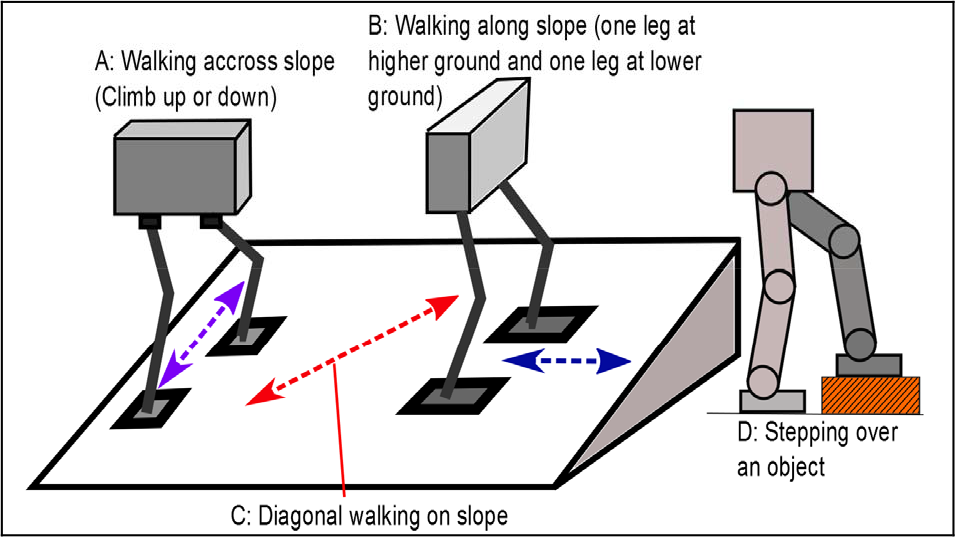
Definitions of walking on a slope and on a step
Walking along a slope has not been investigated yet. For that reason, the main task of this paper is to investigate biped walking along a slope. In the conventional methods, the centre of mass (CoM) is suggested to be brought up or down in order to maintain the same pendulum length at the right foot (RF) and left foot (LF). In this paper, a method known as the dual length linear inverted pendulum method (DLLIPM) is proposed where the CoM always moves in a horizontal way, as shown in Figure 2.
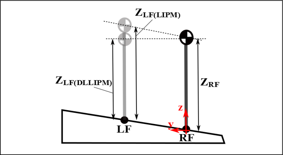
CoM trajectory in the lateral plane for walking along a slope with LIPM and DLLIPM
The conventional method requires extra effort to move the CoM up to the higher ground. In order to avoid this situation, the CoM always moves in a horizontal motion in the proposed method. It is expected that higher ground reaction force (GRF) will occur at the landing foot in the conventional methods, especially when the CoM is moving down from higher to lower ground. On the other hand, when different heights of the CoM are assigned to the RF and LF in DLLIPM, there is a possibility of unsmooth and non-symmetrical pendulum motions. Due to these non-symmetrical pendulum motions, the GRF fluctuation will increase. Therefore, the Newton Raphson algorithm is applied in order to find the optimal parameters for the walking pattern. This will be explained further in Section 4. In this paper, three-dimensional (3D) pattern generation for walking along a slope is investigated. The sagittal and lateral effects are analysed and their synchrony during walking is ensured.
There are several advantages expected from the proposed method. One of the benefits is that, since the CoM in the DLLIPM is maintained horizontally, the GRF is reduced. Less fluctuation of the forces will ensure a more stable walking motion. Besides that, smooth motions, straight walking direction and synchronization between the lateral and sagittal plane are confirmed with the proposed method.
The rest of this paper is organized as follows. In Section 2, the robot platforms are presented. In Section 3, the concept of DLLIPM is explained. The main contribution of this paper is written in Section 4. Simulation results are presented in Section 5. Finally, conclusion and future work are discussed in Section 6.
2. Robot platforms
The proposed method introduced in this paper is applicable to any general bipedal robot platforms. However, in this paper calculations and simulations are based on a bipedal robot called MARI-3 [15]. In order to verify the proposed method, a 3D dynamic simulator known as ROCOS (RObot COntrol Simulator) is used [16]. Figure 3 shows the actual robot and its ROCOS simulation model.

Biped robot MARI-3
One of the advantages of DLLIPM is that it is a general method applicable to any type of bipedal robot platform. However, it is compulsory to calculate the CoM of the robot and it must be able to be tracked during walking. This is essential because all the derivations in this paper are developed based on the dynamics of a linear inverted pendulum, which is assigned to the motion of the CoM. The calculation of the CoM can be done from the kinematics of the robot. A picture of a general biped robot with its centre of mass position is shown in Figure 4. In this paper, the CoM position is controlled.

MARI-3 robot structure
There are two different coordinate systems in this paper. For the trajectory planning, the centre of the landing foot is used as the origin of the coordinate system, where both the RF and LF are repeatedly used as the reference point, one after another. Whereas the origin of the coordinate system during simulations is always located at the centre of the RF at the initial position before walking begins. This coordinate system is known as the world coordinate system.
3. Dual length linear inverted pendulum method (DLLIPM)
DLLIPM is designed based on the LIPM concept [8]. DLLIPM can be used to solve biped walking along a slope or stairs. In both situations, the problems are solved by maintaining the CoM height so that it always moves horizontally. In order to realize this, the DLLIPM is used where the lengths of the pendulum at the RF and the LF are different, unlike in the conventional methods. In conventional methods, the CoM is always in parallel with the slope surface in order to let the height of the pendulum be the same for both feet. The concepts of both conventional and proposed methods are shown in Figure 5 and 6. In these figures, Zlf means the height of the CoM measured from the middle of LF when the CoM is just above the middle of LF vertically. Zrf means the height of the CoM measured from the middle of the RF when the CoM is just above the middle of the RF vertically. In the case of Figure 5b) and 6b), Zlf is also known as Zsp and Zrf is known as Zlp. ‘sp’ and ‘lp’ stand for short pendulum and long pendulum, respectively.

CoM motion of a biped robot on a slope in the lateral plane

CoM motion of a biped robot on a slope in the sagittal plane
3.1 Linear inverted pendulum mode (LIPM)
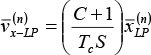
In this sub-section, the equations of the position and velocity of a single linear inverted pendulum are derived [8]. The single linear inverted pendulum models for sagittal and lateral motions are shown in Figures 7 and 8, respectively. In these figures, ‘i’ and ‘f’ stand for initial and final. In Figure 7, the initial position, initial velocity, initial acceleration, final position, final velocity and final acceleration of the CoM in the sagittal plane are shown. Whereas, in Figure 8, the initial position, initial velocity, initial acceleration, final position, final velocity and final acceleration of the CoM in the lateral plane are shown. x(t) and y(t) denote the instantaneous value of the CoM trajectory in the sagittal and lateral planes, correspondingly. Furthermore, S denotes the CoM stride motion between the LF and RF. Whereas Zc denotes the height of the pendulum, from the foot to the CoM position vertically.
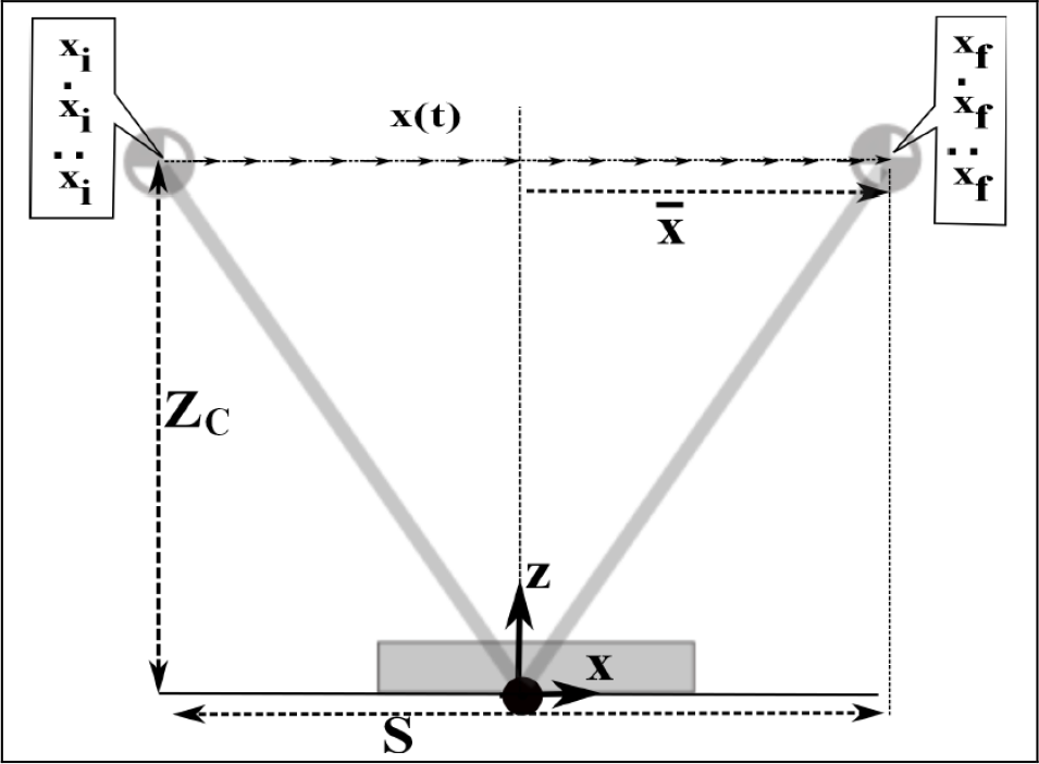
LIPM model for the sagittal plane

LIPM model for the lateral plane
The motion equation of LIPM in the sagittal plane is shown as in (1). The same equation is also applicable for the lateral plane.

3.1.1 Position
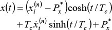
In this sub-section, the derivation of the equation, which is related to position in single linear inverted pendulum model, is shown. From the analytical solution of (1), the equation of the position is obtained as shown in (2).

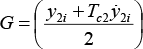
where the value of Tc in (2) is given as in (3).

The position equation shown in (2) is applicable for the sagittal and lateral planes.
3.1.2 Velocity
In this sub-section, the derivation of the equation, which is related to velocity in single linear inverted pendulum model, is shown. The time derivative of (2), gives an equation of the velocity, as shown in (4).

The velocity equation shown in (4) is applicable for the sagittal and lateral planes.
3.2 Trajectory planning method of DLLIPM
DLLIPM trajectory planning consists of 11 steps, as shown in this sub-section. This trajectory planning is based on an LIPM proposed by Kajita et al. with some changes [8].


where

If n is an even number, T:= T+Δtlp.
If n is an odd number, T:= T+Δtsp.


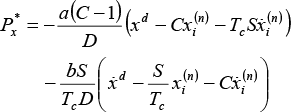
where sx(n) and sy(n) mean the foot strides of the nth step in the sagittal and lateral directions.


If n is an odd number, the final CoM position and the final velocity for the sagittal and lateral planes can be solved in the same way as (13)–(16) but with the respect to the short pendulum.
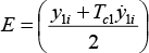
The values of C and S in (14) and (16) are given in (17) and (18) (suppose that the instantaneous time at the end of each single support phase is denoted by tend).


where the values of Tc in (14), (16), (17) and (18) are the same values used in Step 5.
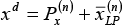


If n is an odd number, the desired final position and desired final velocity of the CoM for the sagittal and lateral planes can be solved in the same way as (19)–(22) but with the respect to the short pendulum.
where D = a(C-1)2 + b(S/Tc)2.
a and b are the weight parameters used in order to minimize the margin of error for position and velocity. The values of Tc, C and S in (23) are the same values as in Step 8. The foot landing modification in the lateral plane can be solved in the same manner as in (23) but with all the values from the lateral plane.
4. DLLIPM with Newton Raphson (proposed method)
It is very important for biped robots to have a symmetrical and smooth motion during walking to reduce the GRF. In order to achieve this, the position, velocity and acceleration between single support phases must be connected smoothly. Furthermore, in 3D walking pattern generation, the sagittal and lateral planes must be synchronized properly. Thus, the use of the Newton Raphson method is proposed and will be presented in this section.
4.1 Biped modelling by DLLIPM for 3-D walking along a slope
For modelling, the long pendulum and short pendulum phases are represented by Phase 1 and Phase 2 as shown in Figure 9 and 10. Phase 1 is defined as the walking cycle of the biped robot when the robot is supported by the foot on the lower slope surface, which means the height of the pendulum in this cycle is referred to as the long pendulum (LP). On the other hand, Phase 2 is defined as the walking cycle of the biped robot when the robot is supported by the foot on the higher slope surface, which means the height of pendulum in this cycle is referred to as the short pendulum (SP).

DLLIPM model for walking along slope in the sagittal plane

DLLIPM model for walking along slope in the lateral plane
4.1.1 Definitions of parameters
All the parameters involved in Figure 9 and 10 are explained and defined in Table 1. Where k in Table 1 is either one or two, which is referred to as Phase 1 or 2, respectively.
Definitions of parameters, where k is 1 or 2 which is referred as phase 1 or 2, respectively

4.1.2 Assumptions
All derivations shown later are based on the following five assumptions:
4.1.3 Constraints
In order to ensure smooth motions and symmetrical pendulums, there are several constraints that must be enforced. In total, there are six constraints, which result in six equations, as shown by (24)-(29). The constraints are listed as follows:
By using the position equations, the pendulums for Phase 1 and 2 are made symmetrical by the following equations:


In order to ensure a smooth trajectory of the velocity and synchronization between the sagittal and lateral planes, a constraint as in (28) is enforced.

In order to ensure a smooth trajectory of the acceleration and synchronization between the sagittal and lateral planes, a constraint as in (29) is enforced.

4.2 Solution of Sx1, Sx2, Sy1, Sy2, Ts1 and Ts2 using the Newton-Raphson method
In order to find a solution for appropriate Sx1, Sx2, Sy1, Sy2, Ts1 and Ts2 parameters, a numerical method known as Newton-Raphson is chosen. There are several steps that need to be taken, which will be discussed further in this section.
4.2.1 Simplification of equations
Before the Newton-Raphson method can be implemented, long and complex equations must be simplified. Therefore, (30)-(39) are defined.


The previous constraint in (24) is realized using (2), as shown in (40).

By substituting (30), (32) and (33) into (40), f1(q) is defined as follows.

The previous constraint in (25) is also realized using (2), as shown in (42).

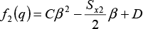
By substituting (31), (34) and (35) into (42), f2(q) is obtained as follows.,
The previous constraint in (26) is realized using (2), as shown in (44).

By substituting (30), (36) and (37) into (44), f3(q) is defined as follows.

The previous constraint in (27) is also realized using (2), as shown in (46).

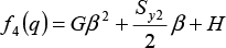
By substituting (31), (38) and (39) into (46), f4(q) is defined as follows.
The previous constraint in (28) is realized using (4), (30)–(39), as shown in (48). (48) is assigned as f5(q).

Then, f5(q) is expanded, as shown in (49).

The previous constraint in (29) is realized using a time derivative of (4), (30)–(39), as simplified in (50). (50) is assigned as f6(q).

Then, f6(q) is defined by expanding (50) as follows.

All the functions are arranged as in (52). In (52) the values of q are the variables or parameters that need to be solved, as shown in (53).


4.2.2 Newton Raphson algorithm
The Newton Raphson method involves a process of iterations. The objective is to obtain the roots from several complex functions. In this method, the roots are calculated using (54).

f'(qn) in (54) is the derivative of the functions, which is obtained as in (55).
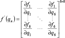
The value of each element in the matrix above is then obtained.
5. Simulation
5.1 The known parameters and initial guess values for Newton Raphson calculations
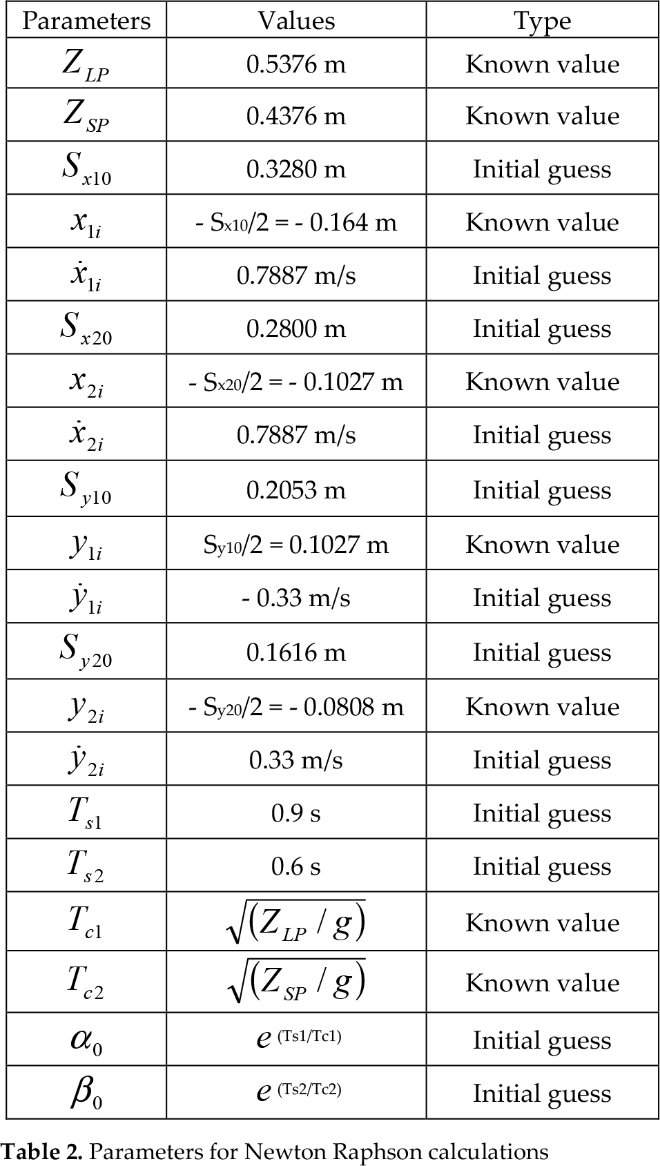
In the Newton Raphson method there are known parameters and initial guess values for iterations that must be given. These parameters are shown in Table 2. The meaning of each parameter in Table 2 can be determined from Table 1.
Parameters for Newton Raphson calculations
5.2 Results of the iterations with the Newton Raphson method
From the values used in Sub-section 5.1, iterations are done by using (54). The results are shown in Figure 10 and 11. α is obtained as 10.5198 at the 5th iteration and β is obtained as 10.2831 at the 4th iteration. Furthermore, Sx1, Sx2, Sy1 and Sy2 are obtained as 0.1842m, 0.2438m, 0.2841m and 0.1287m, correspondingly. During the iterations process of the Newton Raphson method, different initial settings and different numbers of iterations may give different solutions. However, the solutions for all the parameters, α, β, Sx1, Sx2, Sy1 and Sy2 must always be positive. It should not be negative because α and β represent the time, which cannot be negative. Sx1, Sx2, Sy1 and Sy2 are the distance of the centre of mass maximum trajectory, which should also always be positive.

Results of α and β after several iterations by using the Newton Raphson algorithm

Results of Sx1, Sx2, Sy1 and Sy2 after several iterations by using the Newton Raphson algorithm
In order to verify all the functions from the Newton Raphson solutions, Figure 12 is plotted. In this figure, all functions are obtained as ‘0’ values after all the parameters are converged. This validates that all the constraints have been fulfilled.
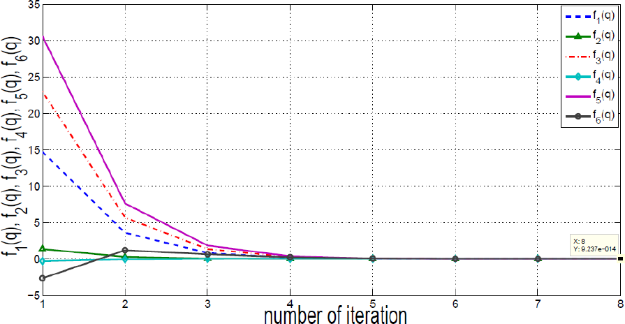
Results of all functions from f1(q) to f6(q) by using the Newton Rahpson algorithm
5.3 Simulation of 3D walking pattern with DLLIPM (without Newton Raphson)
In this sub-section, a simulation of a biped robot walking along a slope with the height of 10cm is presented. All simulations in this paper are done for a slope, which means the floor is not horizontally flat. Therefore, the foot should be made parallel to the slope surface and realized with an orientation command [15]. The strides are decided as in Table 3.
Strides table

Zlp, Δt-lp and Δt-sp are 0.5376m, 0.9s and 0.6s correspondingly. Here, the parameter settings are chosen intuitively without the Newton Raphson method. With these settings, the trajectory planning method in sub-Section 3.2 is used. The result for the sagittal plane is obtained as in Figure 13. The result for lateral plane is shown in Figure 14.
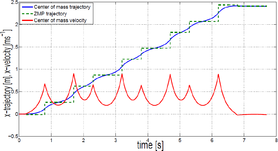
Walking pattern of ten steps in the sagittal plane (without proposed method)

Walking pattern of ten steps in the lateral plane (without proposed method)
As for the sagittal plane, it is noticed from Figure 13 that the CoM position trajectory shown by the blue line is accelerated and decelerated repeatedly. Thus, the impact force may increase. It is also noticed that there are multiple levels of maximum and minimum velocity for the long pendulum and short pendulum cycles. These multiple levels of velocity will create unsmooth motion during walking.
As for the lateral plane, it is observed from Figure 14 that the CoM position trajectory becomes deviated from its initial straight position. The deviated problem is more critical during the first few steps. It is also observed in this figure that the shape of the velocity trajectory, shown by the red line is not symmetrical.
5.4 Simulation of 3D walking pattern with improved DLLIPM (with Newton Raphson)
By using DLLIPM algorithm shown earlier in Sub-section 3.2, the walking pattern for the environment or situation in Sub-section 5.3 is simulated again with the new walking parameters obtained from Sub-section 5.2. The result for the sagittal and lateral planes is obtained as in Figure 15 and 16, respectively.
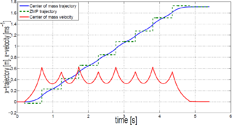
Walking pattern of ten steps in the sagittal plane (with proposed method)

Walking pattern of ten steps in the lateral plane (with proposed method)
As for the sagittal plane, it is noticed in Figure 15 that the trajectory of the CoM does not accelerate and decelerate repeatedly as much as the previous situation, shown in the Figure 13. Thus, the impact force may be reduced. Besides that, it is noticed that the minimum velocity for the long pendulum and short pendulum cycles is now at the same value, which results in a smoother walking motion.
As for the lateral plane, it is observed that the motion of the CoM does not deviate from its initial straight position as shown in Figure 16. Furthermore, it is also noticed from this figure that the problem of the unsymmetrical shape of velocity trajectory has been solved. Smooth trajectories will help a bipedal robot to achieve safer and more stable walking. From all the results illustrated, it is verified that with the proposed method, the biped walking pattern for walking along a slope has been improved.
5.5 Ground reaction force (GRF)
Simulations of biped robot walking with consideration of the lateral and sagittal planes are conducted for walking along a slope. The simulations are conducted for walking with LIPM and DLLIPM approaches, as explained earlier in Figure 5 and 6. In other words, these simulations are done for comparison between the conventional method and the proposed method. In these figures, the RF always lands on the lower slope surface. Whereas the LF always lands on the higher slope surface during walking. The GRF during these walking simulations is measured with the force sensors located at the RF and LF of the biped robot. The results are shown in Figure 17 and 18.
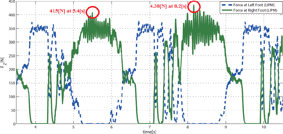
GRF data measured from force sensors during walking simulation (without proposed method)

GRF data measured from force sensors during walking simulation (proposed method)
The solid lines in Figure 17 and 18 represent forces measured at the RF of the biped robot. Furthermore, the dashed lines in these figures are the forces measured at the LF of the biped robot. It is noticed from the red circles shown in Figure 17 that the maximum force fluctuation is 415 [N] at 5.4[s] and 4.38[N] at 8.2[s]. The maximum force fluctuation is reduced to 380[N] at 5.4[s] and 410[N] at 8.3[s] with the proposed method, as shown in Figure 18. These facts demonstrate the effectiveness of the proposed method in order to reduce the GRF.
6. Conclusions and future work
In this paper, a generalized method known as DLLIPM with the Newton Raphson algorithm is proposed in order to determine parameters of 3D biped walking along a slope. By using DLLIPM, different heights of pendulum are applied at the left and right legs.
However, when different heights of pendulum are applied, difficulty occurred in obtaining symmetrical and smooth pendulum motions. Furthermore, synchronization between the sagittal and lateral planes is not confirmed. Therefore, DLLIPM with the Newton Raphson algorithm is proposed in order to solve these problems. As a result, smoother walking trajectories and more symmetrical pendulum motions are achieved. Furthermore, it is verified that the maximum force fluctuation is reduced with the proposed method. In the future, the concept of DLLIPM will be expanded for other possible motions such as diagonal walking, turning on a slope and stairs.
Footnotes
7. Acknowledgements
The authors would like to thank Universiti Teknikal Malaysia Melaka (UTeM) for the funding of this research with grant number PJP/2013/FKE(11C)/S01188 and also to Professor Atsuo Kawamura from Yokohama National University for all the great idea.