
Abstract
A neural network based robust control system design for the trajectory of Autonomous Underwater Vehicles (AUVs) is presented in this paper. Two types of control structure were used to control prescribed trajectories of an AUV. The vehicle was tested with random disturbances while taxiing under water. The results of the simulation showed that the proposed neural network based robust control system has superior performance in adapting to large random disturbances such as underwater flow.
It is proved that this kind of neural predictor could be used in real-time AUV applications.
Nomenclature

1. Introduction
Nowadays, AUVs are widely used for underwater investigations. Son and Kim [1] investigated manoeuvrable control of an underwater vehicle using a combined discrete-event and discrete-time system simulation. The proposed simulation model was established on the basis of discrete-event system specification formalism, representative of a discrete-event system simulation. The proposed approach made it possible to build a simulation-based expert system to support decision-making in the acquisition of an underwater vehicle.
Santhakumar and Asokan analysed dynamic station keeping of an under-actuated flat-fish-type AUV, and proposed a new method of station keeping with the addition of dedicated thrusters [2]. The effect of the additional thrusters on tracking performance was analysed and a modular configuration (using retractable thrusters) was developed. The effects of underwater current magnitudes and angle of incidences on the station keeping performance were also investigated. A comparative analysis of power consumption during station keeping proved the effectiveness of the proposed modular configuration.
An adaptive neuro-fuzzy sliding-mode-based genetic algorithm control system for a remotely operated vehicle with four degrees of freedom was presented by Moghaddam and Bagheri [3]. A set-point controller for autonomous underwater vehicles was proposed by Herman [4]. The controller was expressed in transformed equations of motion with a diagonal inertia matrix. The stability of the proposed control law was proven and the performance of the developed controller was verified via simulation on the underwater vehicle.
Kumar et al. presented a new control scheme for robust trajectory control of underwater vehicles. The effectiveness of the controller was verified through simulations and execution issues were discussed. Adaptive control of low-speed bio-robotic autonomous underwater vehicles in the dive plane using dorsal fins was also considered [5].
Narasimhan and Singh developed an indirect adaptive control system for depth control using dorsal fins. According to the simulation results, the adaptive control system accomplished precise depth control of the bio-robotic autonomous underwater vehicle using dorsal fins, in spite of large uncertainties in the system parameters [6]. Autonomous underwater vehicle control architectures were reviewed and sensor data bus based control architecture was investigated by Kim and Yuh [7].
A wave drift force that severely affects the underwater vehicle in shallow water was examined by Luo et al. [8]. On the basis of wave force analysis, three-dimensional disturbances caused by wavy surge water were measured, and a control system was proposed using least-squares multi-order data fitting polynomial prediction and fuzzy compensation, combined with a PID controller. The experimental results showed that the control system for disturbance of surge and wave was feasible and effective.
A chattering-free sliding-mode controller was developed by Soylu et al. for the trajectory control of remotely operated vehicles. A new approach for thrust allocation was also proposed based on minimizing the largest individual component of the thrust manifold [9]. Bessa et al. [10] developed an adaptive fuzzy sliding mode controller for remotely operated underwater vehicles. Their study was carried out based on the sliding mode control strategy and enhanced by an adaptive fuzzy algorithm for uncertainty/disturbance compensation. The performance of the proposed control structure was also appraised using numerical simulations.
Naik and Singh [11] investigated the problem of suboptimal dive plane control of autonomous underwater vehicles using the state-dependent Riccati equation technique. The simulation results showed that effective depth control was accomplished in spite of the uncertainties in the system parameters and control fin deflection constraints.
In other research, a neuro-fuzzy controller for autonomous underwater vehicles was proposed by Kim and Yuh [12]. Simulation results showed effectiveness of the neuro-fuzzy controller for autonomous underwater vehicles. Akkizidis et al. [13] used a fuzzy-like PD controller for an underwater vehicle, and analysed and presented experimental results. A switched control law for stabilizing an under-actuated underwater vehicle was proposed by Sankaranarayanan et al. [14], and simulation results were presented to validate this. Lapierre [15] designed and verified a diving-control method based on Lyapunov theory and back-stepping techniques. The results of the control system and subsequent simulations demonstrated the performance of the solutions proposed.
The organization of the present paper is as follows. The following section describes some of the theory of AUVs. A proposed robust neural feedback control system is outlined in Section 3. The simulation results are given in Section 4. Finally, conclusions are presented.
2. Dynamics equations of autonomous underwater vehicle
The motion for an underwater vehicle's generalized six-degree of freedom equations is derived under the following assumptions:
The vehicle behaves as a rigid body; The earth's rotation is negligible as far as acceleration of the centre of mass is concerned; The vehicle moves at low speed; The hydrodynamics parameters are constant;
The equations of motion for an underwater vehicle can be represented as in [16, 17]:

where

where J(η) is the kinematics transformation matrix and η = (x,y,z,φ,θ,ψ) T . The linear steering equations of motion are:

where the components of the matrix are as follows:

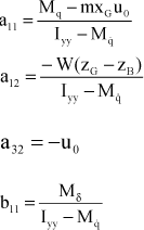
The linearized forms for equations of the AUV motion containing heave and pitch are as follows:
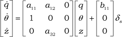
where the components of the matrix are as follows:
Schematic representation of the AUV system with coordinates is shown in Figure 1. The hydrodynamics parameters and the AUV parameters are given in Table 1.
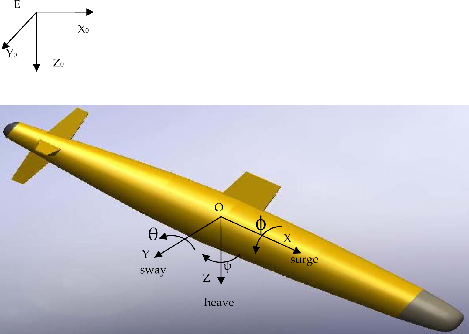
Schematic representation of the AUV system with coordinates
The hydrodynamics parameters and the AUV parameters

3. Robust Neural Feedback Control System (RNFCS)
A designed control system is employed to control the trajectory of the AUV. The purpose of this proposed control system is to provide the appropriate control action. The mathematical expression of the force of the RNF control system is given by:

where

where KP, KD and R are the proposed control system parameters and are empirically set to KP = 10, KD=7 and R = 0.0001. In the following equation, e(t) is the control error:

where yr(t) is the reference input signal and y(t) is the system output signal. Neural network structure is shown in Figure 2. The second part of the control input for the proposed control system is explained in the following subsection.

Schematic representation of the neural network model
3.1 Neural controller
A neural controller with Resilient Back-propagation Algorithm is one popular neural network structure for control and prediction. Fundamentally, two steps are involved when using this control: system identification and control design. The identification stage of this control is to train a neural network to present the forward dynamics of the plant. The neural network model of the plant that needs to be controlled is developed using two sub-networks for the model approximation. The neural model is as follows:

where y(t) is the system output, u(t) is the system input and d is the relative degree (d≥2). Multilayer neural networks can be used to identify the function F. The identification model has the form:

where ŷ(t + d) is the estimate of y(t + d). Identification is carried out at every instant t by adjusting the parameters of the neural network using the error e(t) = ŷ(t) - y(t). For a system output, y(t+d) is used, and for a reference trajectory yr(t+d).

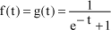
f and g are activation functions of the hidden layer in the first and second sub-networks, respectively, as follows:
For each sub-network, the linear activation function uses the output layer. The controller output will have the form:

Using the equation directly causes a realization problem based on the output at the same time, y(t). So, instead:

Using Eq. (13):

Figures 3 and 4 represent the neural plant model identification and the neural controller, respectively. The proposed RNF control system architecture is shown in Figure 5. The neural network training parameters are given in Table 2. The Resilient Back-propagation algorithm is used to adjust the weights of the neural network.
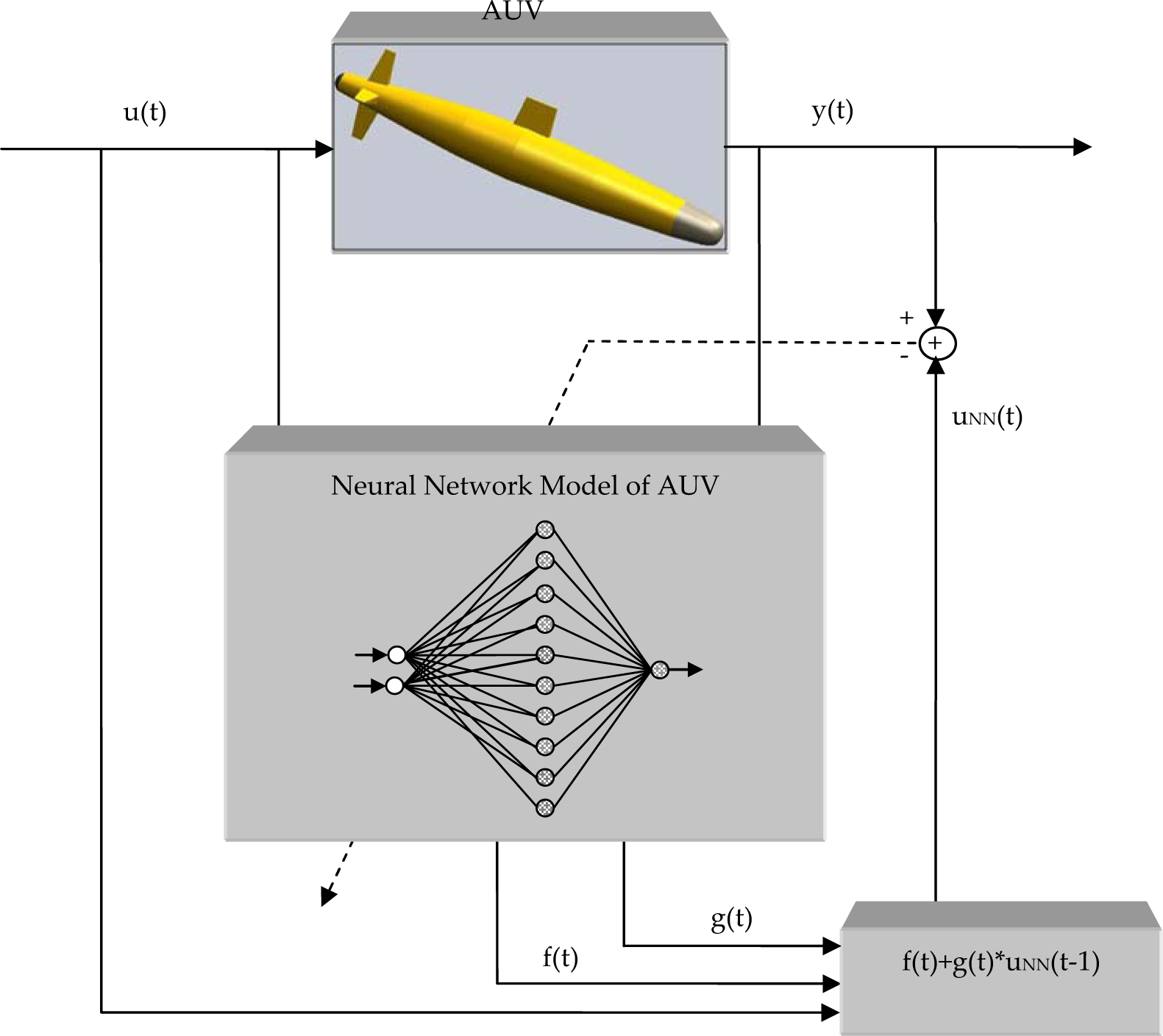
Neural controller plant model identification
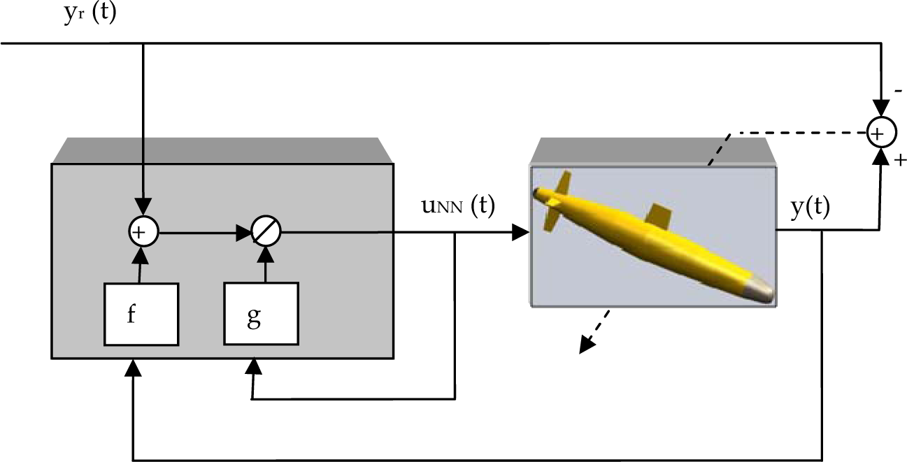
Neural controller
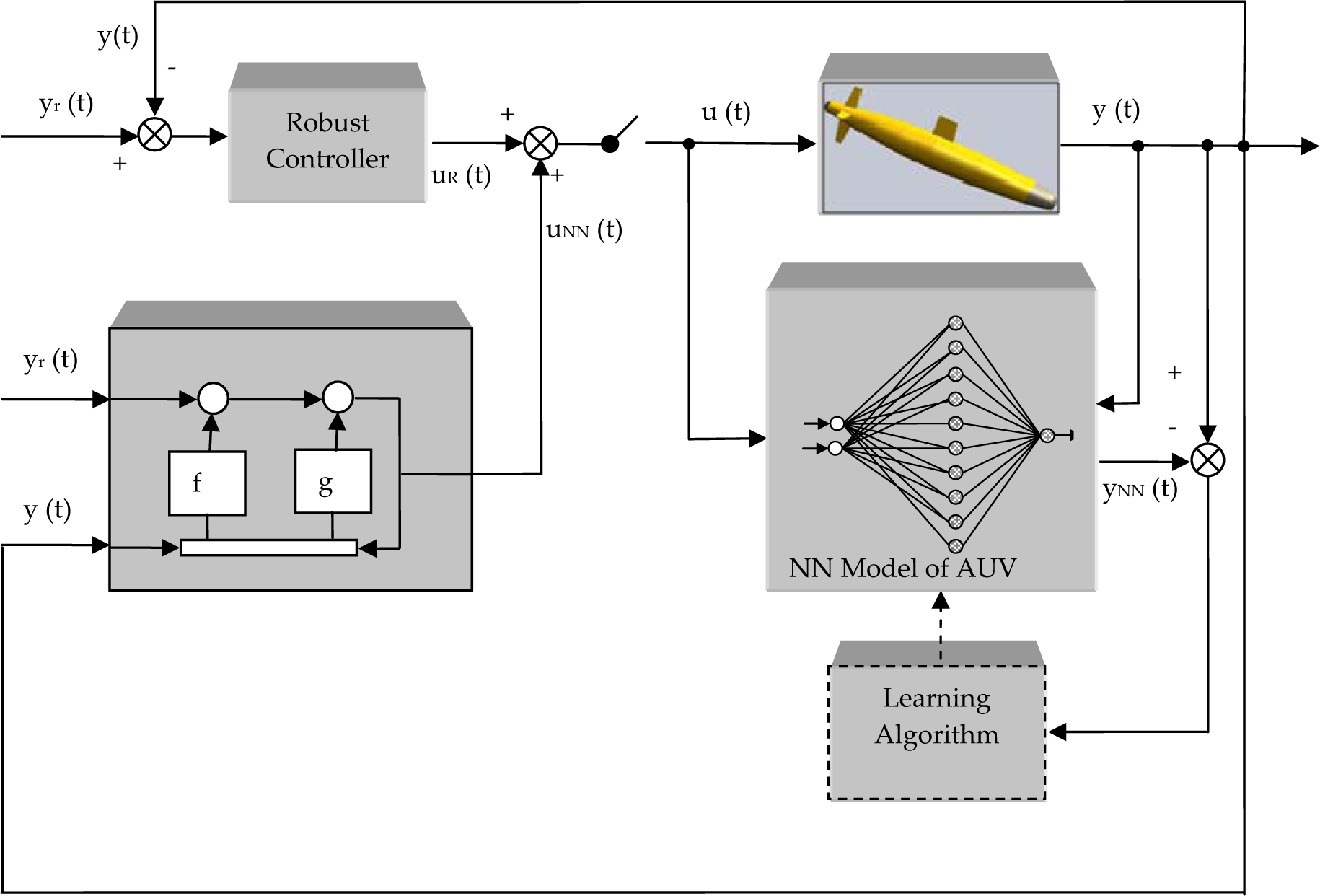
Proposed RNF control system architecture
The neural network training parameters

3.1.1 Resilient Back-propagation Algorithm (RPROP)
The Resilient Back-propagation Algorithm is a local adaptive learning scheme performing supervised batch learning in feed-forward neural networks. The basic principle of this algorithm is to eliminate the harmful influence of the partial derivative's size on the weight step. As a consequence, only the sign of the derivative is considered to indicate the direction of the weight update. This algorithm typically uses a sigmoid function in the hidden layers and a linear function in the output layer. Here, Wij is the weight matrix, and Δ ij (t) is the update value for each weight. A second learning rule is introduced which determines the evolution of the update value Δ ij (t). This estimation is based on the observed behaviour of the partial derivative during two successive weight-steps:
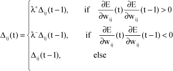
where

The adaptation rule works as follows. Every time the partial derivative of the corresponding weight Wij changes its sign, which indicates that the last update was too big and the algorithm has jumped over a local minimum, the update value Δ ij (t) is decreased by the factor λ-. If the derivative retains its sign, the update value is slightly increased in order to accelerate convergence in shallow regions. Once the update value for each weight is adapted, the weight-update itself follows a very simple rule: if the derivative is positive (increasing error), the weight is decreased by its update-value; if the derivative is negative, the update value is added. This is formulated as follows:


However, there is one exception. If the partial derivative changes sign, i.e., the previous step is too large and the minimum is missed, the previous weight-update is reverted to:

Due to this ‘backtracking’ weight-step, the derivative is supposed to change its sign once again in the following step. In order to avoid a double punishment of the update value, there should be no adaptation of the update value in the succeeding step. In practice, this can be achieved by setting

Hence, the partial derivatives of the errors must be accumulated for all P training patterns. This means that the weights are updated only after the presentation of all training patterns. The α (weight-decay) parameter determines the relationship of two goals, namely to reduce the output error (the standard goal) and to reduce the size of weights (to improve generalization). The composite error function is:

For comparison purposes, the classical PID controller was used for trajectory control of the AUV. The PID controller was initially tuned using the Ziegler-Nichols method; the PID parameters are given in Table 3.
The PID gain parameters with Zeigler-Nichols method

4. Simulation results
This section presents simulation results of the AUV system with neural network based controller for rudder deflection, yaw angle, theta angle and depth change. Figures 6(a)–(c) show the responses of these parameters without any controller and in the presence of a PID controller and the proposed RNF control system, respectively.

Rudder deflection of AUV for sinusoidal input signal (a) Uncontrolled response (b) PID controller response, and (c) RNF control system response
Figure 6(a) shows the rudder deflection of the AUV for sinusoidal input signal. The response of the AUV unstable behaviour (shown with dashed lines) is also seen in Figure 6(a). Figure 6(b) depicts the response of rudder deflection of the AUV for sinusoidal input signal using the standard PID controller. As seen in the Figure, the system response does not show unstable behaviour, but the desired sinusoidal input signal does not follow. The results show that the proposed RNF control system has better performance in terms of adapting a sinusoidal input signal. Figure 7(a) shows rudder deflection of the AUV for a random input signal; in Figure 6(a) the response of the AUV is unstable behaviour. The result of the PID controller for rudder deflection of the AUV is shown in Figure 7(b). As seen in Figure 7(b), the rudder deflection response of the AUV with the PID controller does not track the desired random input signal. Figure 7(c) shows the result of the RNF control system. The graph shows a small overshoot error between the desired random input signal and the proposed control system.

Rudder deflection of AUV for random input signal (a) Uncontrolled response (b) PID controller response, and (c) RNF control system response
Figures 8(a), (b) and (c) indicate the yaw angle result without any controller and with the PID controller and the proposed RNF control system for a sinusoidal input signal. As seen in the Figure s, the yaw angle response of the AUV does not show unstable behaviour, whereas the proposed RNF control system exactly follows the desired sinusoidal input signal.

Yaw angle of AUV for sinusoidal input signal (a) Uncontrolled response (b) PID controller response, and (c) RNF control system response
Figures 9(a), (b) and (c) show the yaw angle without any controller, and with the standard PID controller and the proposed RNF control system in the case of a random input signal. As depicted in Figure 9(c), some differences can be seen between the proposed control system response and the desired random input signal.

Yaw angle of AUV for random input signal (a) Uncontrolled response (b) PID controller response, and (c) RNF control system response
The response of the theta angle of the AUV for a sinusoidal input signal is given in Figures 10(a), (b) and (c). As shown in the Figure s, the proposed control system has the best performance in terms of adapting to the sinusoidal input signal. Figures 11(a), (b) and (c) present the response of the theta angle for a random input signal. The results prove that the proposed RNF control system is suitable for controlling the theta angle.

Theta angle of AUV for sinusoidal input signal (a) Uncontrolled response (b) PID controller response, and (c) RNF control system response

Theta angle of AUV for random input signal (a) Uncontrolled response (b) PID controller response, and (c) RNF control system response
Finally, Figures 12(a), (b) and (c) show the results of the AUV?s depth change. According to simulation results, the proposed control system has excellent performance for controlling the AUV parameters.

Depth change of AUV (a) Uncontrolled response (b) PID controller response, and (c) RNF control system response
5. Conclusions
A robust control system with a neural network was designed for trajectory controlling of an AUV system. Four parameters of the system were analysed and controlled by the proposed control system structure.
For comparison, the standard PID controller, tuned using the Ziegler-Nichols method, was also employed to control the AUV. The results of both control systems showed that the use of the proposed robust neural feedback control system was effective in controlling the AUV and more robust than the PID controller. The strong performance of the proposed RNF control system was due to the inclusion of both linear and non-linear neurons in the network. As shown by the simulation results, the proposed control system can effectively track a given trajectory for experimental applications.