
Abstract
The future mobility of urban areas is changing constantly; ideally, vehicles should be able to drive autonomously through traffic. Unfortunately, autonomous vehicles are not yet fully capable of matching human performance. Therefore, the teleoperation of vehicles presents a solution for this task. During teleoperation, a human driver is responsible for driving the vehicle using information transmitted from the vehicle to a working station. Unfortunately, because of the artificial environment in which the operator is located, it is very difficult to achieve high telepresence and accurate speed estimation. It is known that in order to safely drive a vehicle, it is very important to be able to correctly estimate the vehicle's speed. This paper presents a study conducted to quantify the speed perception tendency of a human operator at the working station. Additionally, it is shown that a training process can at least temporarily improve speed perception. Furthermore, the implementation of zoom blur to increase optical flow is shown to positively influence speed perception. Four hypotheses are defined and analysed to study speed perception at an operator's working station. The results are presented and discussed.
Introduction
The world's population is growing rapidly and the number of megacities with a population above ten million will probably double in the next few decades [1], which will have an enormous influence on individual daily mobility. The future mobility of urban areas will most likely consist of integrated mobility concepts, where the vehicle is only one means of transport among others and might be shared with other users through forms of car-sharing concepts [2]. Ideally, the vehicle would be driven autonomously to the customer. Despite the fast progress achieved in the research field of autonomous vehicles, machine perception continues to be unable to match human perception skills. Many events, like the DARPA Urban Challenges, show not only the achievements but also the limitations of fully autonomous vehicles [3–6]. Research in the field of autonomous vehicles has led to the conclusion that autonomous vehicles on urban public roads are not yet feasible [7].
On the other hand, the driverless and automated distribution of vehicles can be achieved through teleoperation. Thanks to large amounts of experience and their capability to predict and anticipate events [6][8], human beings are capable of performing quite well in driving-related tasks and it is therefore reasonable to keep them in the overall loop. The basic concepts of vehicle teleoperation are being studied and implemented at the Institute of Automotive Technology.
Because the operator is spatially separated from the teleoperated road vehicle, further problems arise in the implementation of such a concept. One of the major problems is that the operator has difficulty estimating the speed of the vehicle while steering it. This greatly influences the operator's driving performance and safety. Accordingly, since being able to estimate the velocity correctly is an essential aspect of vehicle driving, as shown in [9], driving at inappropriate speeds is the main cause of accidents. It is therefore of great importance to study and deal with the limited speed perception of a human operator.
State of the art
In order to design a teleoperated system, it is necessary to study the influencing variables of human driving. Although a human driver normally uses four relevant senses, the most important ones for the driving task are the visual and the aural senses [10][11], even though haptic and vestibular senses are also partially involved. Both of these senses enable the human operator to make a timing and position-related prediction, making them the most important for the highly dynamic traffic [12] in road situations where teleoperation would be applied. However, there are limitations at the operator workstation, especially in terms of the human senses. This is because the transmission of sound from the vehicle to the workstation has not yet been implemented. Furthermore, motion, used for modelling acceleration and forces, is missing in the workstation, which further limits the human senses. It is already well known that the situation awareness of the operator plays an important role in the safety of the teleoperated vehicle and accidents become more frequent if the situation awareness is less than ideal [13]. As mentioned above, the correct estimation of velocity by the human operator is essential.
It is important to mention the perception of one's own movement. Parallel to the perception of motion in the world, the awareness of one's own motion in the world is of interest. Regarding the above-mentioned awareness, Gibson discussed the phenomenon of visual kinesthesis. He suggested that “vision is kinesthetic in that it registers movements of the body just as much as does the muscle-joint-skin system and the inner ear system. Vision picks up both movements of the whole body relative to the ground and movement of a member of the body relative to the whole” [14, p.183]. Gibson mentioned that visual kinesthesis goes along with muscular kinesthesis and that the doctrine that vision obtains only external information is false.
Furthermore, it was determined that the visual sense is the most influential in speed perception [15][16]. Moreover, it was also proved that the aural sense is essential for speed perception [17], while haptic feedback has almost no influence [15].
Studies in the field of speed perception in road vehicles have been a common topic for researchers. Especially extensive is the study by Bubb [18], in which different test subjects estimate speed under different circumstances, i.e., as the driver in his or her own vehicle, as the co-driver in an unknown vehicle and directly estimating speed in a video simulator. Similarly, Recarte et al. [19] conducted tests with drivers and co-drivers and compared the results. In both studies, the results showed a strong tendency toward under-estimation, showing an improvement in estimations at higher velocities.
In order to influence the sense of speed by modifying the field of view (FOV), several studies have been conducted; most of them implemented using driving simulators. Mourat et al. [20] showed that the field of view in the driving simulator has an immense influence on test subjects' estimation of speed. Other studies, [21–23], all came to the same result. It was determined that the larger the field of view was, the faster the estimated speed.
On the other hand, there are few studies related to the use of the blur effect in moving pictures to influence the sense of speed. This approach is already used in many computer games and in static pictures to produce the effect of motion.
Due to the architecture of the human eye, the eye is also capable of detecting movements in the peripheral visual field, as mentioned in [24]. During movement, observers see the environment drifting past them, as shown in Figure 1 [25][26]. This is emphasized through the vectors shown directly in the figure. From point A, which is also known as the “focus of expansion” and lies far away relative to the observer, the vectors flow apart and become larger in perception as the distance to the observer decreases. Furthermore, the perceived speed increases with increasing distance toward the edges. This behaviour is known as optical flow.

View of the vector field that an observer perceives while crossing a bridge [26]
Since the advent of photography, it has been known that blur effects are able to produce a sensation of speed. However, in the application of teleoperated road vehicles, it is undesirable for the whole picture to become blurred, since the visibility of the driver should remain unobstructed. Therefore, the blur effect will be applied only to the outer ranges of the picture. Two methods are introduced: motion blur and zoom blur. Finally, studies are conducted with test subjects using the zoom blur method to establish the effects of zoom blur on speed perception.
Motion blur
In this method, two or more pictures (or frames) of the video are superimposed. In order to minimize the transition between frames and improve the visibility, older pictures can be blended in using transparency. Optimally, the older the picture is, the stronger the transparency. Figure 2 shows an example of the effect of motion blur at different speeds.

Example of an arrow using motion blur at different speeds
The biggest advantage of motion blur is that only moving objects will become blurred. The disadvantage is the need for multiple images, meaning that it cannot be achieved using a single picture. In order to achieve smooth transitions, a higher frame rate is necessary, especially when dealing with high speeds, where the differences between each frame are too strong and no smooth transition can be achieved. An example can be seen in Figure 3.
This method offers the advantage that a single frame can be used to achieve the blur effect. It uses the basic idea of taking the same frame, slightly stretching it, overlaying it on the original frame and removing the side margins. This process can be repeated indefinitely to produce stronger effects. With higher transparency, smoother transitions can be achieved. The intensity of the blur depends on the degree of stretching and on the number of stretched overlaid frames. The disadvantage of this approach is that all objects in the side margins become distorted, regardless of speed. Figure 4 shows an example of a real camera frame using zoom blur.

Example of real camera frame using motion blur

Example of real camera frame using zoom blur
It can be argued that zoom blur produces a blur that radiates to the margins from the centre. However, this type of blur produces a perceived forward motion into the image. This effect affects the amount of speed towards the centre of the image [27]. Additionally, due to the limited bandwidth provided by cellular networks for video transmission, only a limited frame rate can be achieved. Considering that differences at high speeds could be too strong and therefore no smooth transition could be achieved, that the main focus of the study is perceived speed and the fact that zoom blur is easy to implement, zoom blur was chosen for this study. The zoom blur effect was created from the centre of the field of view in horizontal directions, thus the direction of travel was towards the centre of the visual field.
Motion blur presents advantages in comparison with zoom blur regarding perception of speed during self-motion. Even though motion blur would provide more realistic images for the operator, due to technical limitations zoom blur was used. The technical limitations include limited bandwidth and the capability of capturing images at a higher frame rate. With a frame rate of 25 fps and a moving speed of, for example, 50km/h, a frame could be captured every 0.55 metres. When overlapping these to create motion blur, tests showed an unrealistic perception.
On the vehicle we have a five cameras system looking to the front, which are displayed on the operator working station as shown in Figure 5. Because of the importance of the middle camera for the driving task, it remains unprocessed so as not to lose important information. The side videos are used to compute the zoom blur effect. The higher the blur parameter [%] is, the higher the blur effect becomes. The blur parameter influences the degree of blur and also the position at which the blur effect starts. The higher the blur parameter is, the closer to the centre of the video the effect begins. A 100% blur parameter would correspond to a blur effect on the four side videos, while an 80% blur effect would cover in total most of the side videos, while the centre-sides videos would only be blurred to a certain degree. This can be seen in Figure 6 and Figure 7.

Five cameras setup at the operator working station

Visualization of the left cameras with 80% blur parameter

Visualization of the left cameras with 100% blur parameter
This study is built on various other studies, including the study by Bubb [18], which provides a great deal of information regarding speed perception in real vehicles and the relationship between speed perception and various sensory channels. The study by Recarte et al. [19] offers results from the comparison between the speed perceptions of the driver and the passenger. This study is based on the abovementioned studies and the study conducted by Conchillo et al. [28].
As already mentioned, studies showed that many test subjects present a tendency toward under-estimation. Therefore, it is the goal of this study to accurately comprehend the perception of speed and improve it. In our application, under-estimation of speed is seen as critical, because the driver would then tend to increase speed. Conversely, an over-estimation would tend to produce a decrease in speed, which could lead to obstructions in traffic but does not present a safety-critical situation. Consequently, the following questions address the problems:
How good is the speed perception of the test subject at using the working station without practice? Does the “learning effect” at the working station influence speed perception? How does the zoom blur effect at the side margins influence the test subject? Which parameters are meaningful for the zoom blur effect?
It should be noted that the zoom blur effect is only used to increase the perceived speed, since this method intensifies the optical flow and therefore is unable to decrease the perceived speed. For the experiment, all measured data is the assertion of the test subjects. Additionally, results are also obtained from demographical surveys. Four hypotheses were defined, which correspond to the abovementioned questions:
NH: The test subjects guess the speed correctly within a defined tolerance. AH: The test subjects under-estimate or over-estimate the speed outside the defined tolerance.
NH: The learning effect does not have any effect on the speed perception of the test subjects at the working station. AH: The learning effect does have an effect on the speed perception of the test subjects at the working station.
NH: Zoom blur does not have any negative effects on the speed perception of the test subjects at the working station. AH: Zoom blur has positive effects on the speed perception of the test subjects at the working station.
NH: Meaningful parameters for the zoom blur are the same for all test subjects. AH: Meaningful parameters for the zoom blur are different for each test subject,
where “NH” stands for Null Hypothesis and “AH” stands for Alternative Hypothesis. All of the mentioned hypotheses are studied by conducting tests where the test subject is asked to guess the speed of a pre-determined sequence of videos. Here it should be noted that prerecorded videos were used so that the experiment remains reproducible and to guarantee that the velocity that was seen by each test subject remains constant. Additionally, the main focus of each test subject should be on the perception itself and they should not be distracted by other activities. Each test person is given an introduction to the study where the important aspects of the study are explained. The subject then completes a survey consisting of demographical questions. Afterwards, the subject assumes his or her position at the working station and begins the study. The complete study consists of five phases:
Duration: about five minutes.
Each test subject is presented with eight different videos, each taken at a pre-determined speed. The test subject then needs to guess the speed at which the vehicle was driving on the videos, without any previous knowledge.
Duration: about five minutes.
This phase can also be called the “learning” phase. The goal is to help the test subject better assimilate the artificial environment at the working station. The test subject is shown the same videos as in Phase 1, but this time the correct driving speed is communicated to the test person. The original guess is also communicated, in case the test person no longer remembers it.
Duration: about five minutes.
After the “learning” phase in Phase 2, the test subject proceeds with another guessing phase. The goal is to test the learning effect on the test subjects. The procedure is exactly the same as in Phase 1, but with different speeds shown.
Duration: about five minutes.
In this phase, two groups are created, Group A and Group B. According to which group the test subject belongs to, Phase 4 differs. Test subjects in Group B are shown a test video in which zoom blur is shown and its settings are explained. Afterward, the test subjects are shown videos with different speeds from those in Phase 1. Any errors in the guessing from Phase 1 are communicated and the test subject is allowed to parameterize the zoom blur in order to achieve a subjective perception of the correct speed using a standard keyboard. It should be noted that there is a possibility that the test subject did not under-estimate the speed. Nevertheless, the option to use zoom blur was also offered to those test subjects. The test subjects in Group A wait for the duration of Phase 4 in order to keep the duration of the study equal for both groups. During Phase 4, the Institute of Automotive Technology is shown to the test subjects in Group A.
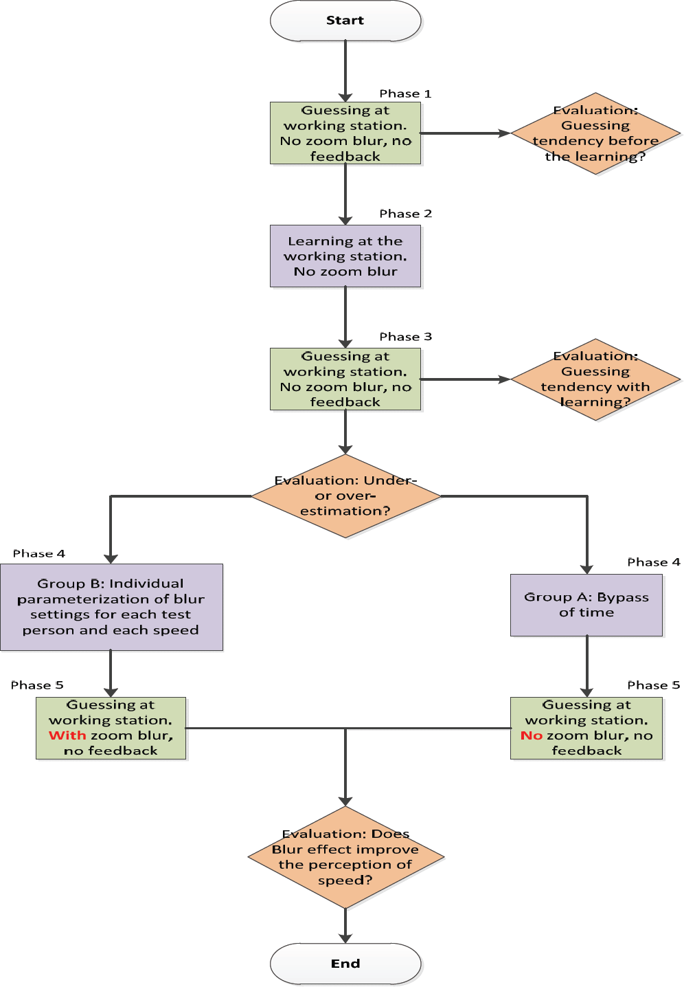
Flow chart of the experiment procedure
The reason for the distinction between Group A and Group B was to have a control group, in order to achieve a comparison between using and not using the zoom blur.
Duration: about five minutes.
The last phase is the same for all subjects. It is identical to Phase 1, with the difference that the same videos were shown as in Phase 3, but in reverse order.
Figure 8 shows a flow chart of the experimental procedure. With the current setup, the test subjects do not have any other type of feedback besides optical feedback. Our intent is to investigate the effect of zoom blur on the optical sensory channel. Therefore caution should be exercised when directly comparing results from this study with results from studies using vehicles or driving simulators.
For the application of teleoperated vehicles the speeds that are driven at in urban areas are of special interest, mainly between 0km/h and 60km/h. In order to achieve a more general applicability of the study, the speed spectrum was set between 0 and 100km/h. In order to avoid speed guesses rounded to multiples of 10km/h, it is explicitly explained that the speeds were measured in 1km/h steps and can therefore be used for the estimation. The guess error is defined as the difference between the real speed and the guessed speed. Here, a positive error value corresponds to an under-estimation and consequently a negative error value corresponds to an over-estimation.
The speeds shown to the test subjects are based on the study by Bubb [18]. In each video showing a different speed, there is a ten second period in which the previous speed in the corresponding cycle is driven, followed by a five second acceleration or deceleration period before achieving the goal speed. The main reason for doing this is due to the effect of differences in the speed perceived. It is known that visual systems adapt to the prevailing image conditions [29]. In other words, a subject who drives at a constant speed for a prolonged time may be subject to a reduction in the perceived speed, but on the other hand, they may be subject to improvement in the sensitivity to changes in the prevailing speed. Therefore, the previous period is shown for ten seconds and in a five second acceleration or deceleration period the test speed is achieved. A buffer of an extra five seconds is reserved before the test person guesses the speed. The speeds shown are provided in Table 1. Different cycles are used for different test groups. It should be noted that the first speed of each cycle, shown in parenthesis, is used only for the abovementioned ten second period before acceleration and is not intended to be guessed by the test persons.
Speeds and cycles used in the study

Speeds and cycles used in the study
In order to improve consistency, all videos of the various speeds were recorded on the same test route, in our case on the FS20 highway north of Munich, between Dietersheim and Eching. These videos are replayed during the study and shown to the test subjects.
For Phase 4, where the test subjects in Group B are given the option of parameterizing the zoom blur settings as deemed appropriate, a standard keyboard was provided, in which two keys were used to increase or decrease the effect of zoom blur.
A total of 30 test subjects participated in this study. This number was chosen because it is a standard reference value in studies with these types of experiments [12]. The only prerequisite for participating in the study was that the subject possesses a class B driving license. The group consisted of 26 men and 4 women, with the youngest person being 19 years old and the eldest 41, with a mean age of 23.2 and a standard deviation of 4 years. The test subjects had held a driving license for a mean duration of 5.6 years and drive an average of 8755km per year. No test subject had an aural disability or limited sight, but eight subjects were required to wear glasses while driving. These test subjects were asked to also wear the glasses during the study.
Results and evaluation
The above hypotheses and the results of the study are presented in the following section. The questions are then answered with an analysis of the results.
For the results, it should be noted that a definition of “good guessing” is needed. In this study, based on the definition by Bubb [18], the definition of “good guesser” was a guessing error of ±4km/h.
From the data obtained from the 30 test subjects in Phase 1 (shown in Table 2) there is a tendency towards under-estimation, which also confirms the results of other studies.
Guess error in Phase 1 at different speeds

Guess error in Phase 1 at different speeds

Average guess error for different speeds in Phase 1 with a linear approximation
In Figure 9 it can be seen that in general, there is a tendency to under-estimate. There is in most cases a positive average speed error, meaning that there is a tendency towards under-estimation of the real speed. A regression analysis showed an x-variable coefficient of 0.766498386 and a y-intercept of 15.57701895, with a R2 coefficient of determination of 0.710393791. The correlation coefficient between real speeds and speed guesses is 0.707 (Kendall-Tau) with a significance level of 0.01. Here, the tendency towards under- or over-estimation is of interest and not directly the absolute value, even though there were large standard deviations.
Additionally, it was tested whether the demographical aspects of the test subjects influence their speed perception. The features tested were age, annual mileage and duration of holding a driving license. Groups were created for test subjects younger than 22 years, who therefore held their driving license for a maximum time period of three years and for test subjects older than 22 years, who had held a license for longer than three years. These groups can be seen as non-experienced and experienced drivers.
Here, in Phase 1, a significant difference between the mean values could be detected (error probability p = 2.6%). The younger test subjects (non-experienced) had a mean error of −0.72km/h and the older test subjects (experienced) had a mean error of 3.14km/h, as can be seen in Table 3.
Comparison between non-experienced and experienced drivers for Phase 1
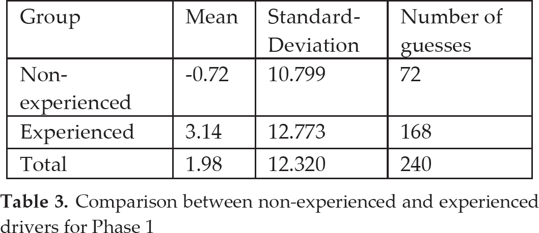
Due to the results from Phase 1 discussed above, Null Hypothesis A is rejected and Alternative Hypothesis A “The test persons under-estimate or over-estimate the speed outside the defined tolerance” is accepted.
It was shown in the previous section that there is a general tendency towards under-estimation of speed. The next step is to analyse whether the learning effect, conducted during Phase 2, has any influence on the speed guessing of the test subjects. Here, the results of the guesses in Phase 3 will be analysed.
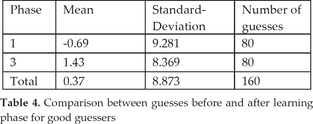
Firstly, the test subjects are divided into three groups, according to the guess errors from Phase 1. The group of “good guessers” are the ones with an average guess error between −4km/h and 4km/h. This group includes a total of ten test subjects. The second group, the “under-estimating guessers,” consists of the subjects with an average guess error above 4km/h and to which 12 test subjects belong. The third group, the “over-estimating guessers,” consists of subjects with an average guess error below −4km/h and to which eight test subjects belong. The “good guessers” achieved good results in Phase 1; with an average guess error of −0.69km/h. It can be said that an error at this level cannot be further improved. Nevertheless, during Phase 3, the test subjects were able to stay at the same level, where an average error of 1.43km/h was achieved. The “under-estimating guessers” achieved an average guess error of 10.69km/h in Phase 1. They were able to improve their performance through the learning phase, reducing the guess error to 2.21km/h. Similarly, the eight test subjects belonging to the “over-estimating guessers,” who achieved an average guess error of −7.73km/h in Phase 1, were able to improve their guess error after the learning phase to an average error of 1.14km/h, which shows a highly significant change.
Table 4, Table 5 and Table 6 show the means, standard deviations and the number of guesses for the three groups, good guessers, under-estimated guessers and over-estimated guessers, respectively. In each case, a T-Test was conducted to see the significance, with significance p-values of p = 0.370, p = 9.887 · 10−19 and p = 1.613 · 10−13 respectively. Therefore, for the good guessers, no significant difference could be established between Phase 1 and Phase 3, but for under-estimated and over-estimated guesses, an improvement could be established.
Comparison between guesses before and after learning phase for good guessers
Comparison between guesses before and after learning phase for under-estimated guessers

Comparison between guesses before and after learning phase for over-estimated guessers

Figure 10 shows the influence of the learning effect on the average error rate. It can be clearly seen that the average guess error improved with the learning phase. Furthermore, the groups of “good guessers” and “over-estimating guessers” corrected their tendency to over-estimate to an under-estimating error, which is considered non-critical.
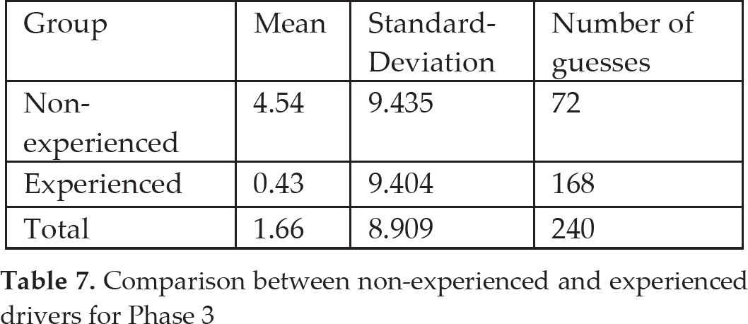
Considering the demographical differences and the two groups consisting of non-experienced and experienced drivers, differences can be recognized. In Phase 1, the experienced test subjects tended to under-estimate, while the non-experienced drivers made very accurate guesses. However, after the learning phase, the result is reversed. The experienced drives made accurate guesses, while the non-experienced test persons under-estimated the speed. Table 7 shows the comparison between non-experienced and experienced drivers.
The results of this analysis lead to the rejection of Null Hypothesis B, meaning that the learning phase does have a highly significant influence on speed perception at the working station.

Influence of learning effect on the guess error
Comparison between non-experienced and experienced drivers for Phase 3
In order to analyse this question, it is necessary to divide the test subjects into two groups, Group A and Group B, as already explained. It is important to clarify whether there are any differences between these groups. The test subjects in Group A guessed the speed in Phase 1 with an average guess error of 1.13km/h and test subjects in Group B guessed the speed in Phase 1 with an average error of 2.83km/h. The variance analysis shows that there is no significant difference. However, it should be noted that there is a significant difference between guesses from Group A in Phase 1 and Phase 5 (t = 6.652 · 10−7) and also a significant difference between guesses in Phase 3 and Phase 5 (t = 0.001).
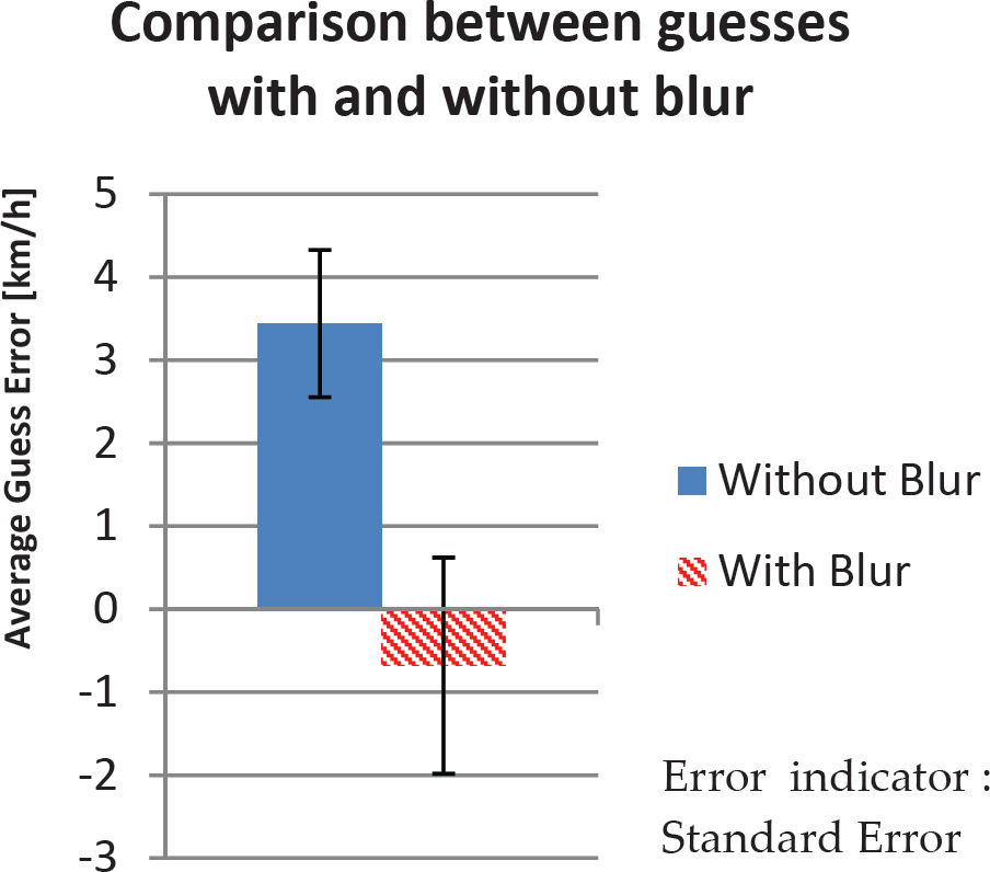
The test subjects parameterized the zoom blur settings during Phase 4 according to each subjective opinion. 13 test subjects of a total of 15 subjects belonging to Group B showed under-estimated guesses in Phase 1. Two of the test subjects never under-estimated, therefore it is not meaningful to use blur and are therefore considered together with Group A. Comparing the guesses in Phase 5 between test subjects from Group B, where blur was used, to the guesses by test subjects from Group A, where blur was not present, a significant difference can be seen (error probability p = 2.4%). The test subjects without zoom blur had an average guess error of 3.44km/h, whereas the test subjects with zoom blur had an average guess error of −0.68km/h. Furthermore, the maximal guess errors by the test subjects in Group B with zoom blur are much smaller compared to the ones without blur. Table 8 and Figure 11 show a comparison of the guesses with and without zoom blur.
Comparison between guesses with and without blur in Phase 5

Influence of zoom blur on the guess error
Additionally, a regression test for the subjects of Group B was conducted for Phase 3 and for Phase 5. In Phase 3 the x-variable coefficient is 0.87300718 and the y-intercept is 10.2237839, with an R2 coefficient of determination of 0.83119047, while in Phase 5 the x-variable coefficient is 0.89982096 and the y-intercept is 7.48560832, with an R2 coefficient of determination of 0.83762969. This further shows an improvement using zoom blur under the condition that the parameters are subject to each individual.
It is very interesting to note that after the guesses in Phase 5, the test subjects were asked whether they felt that zoom blur had helped them improve the guessing process. Figure 12 shows the results of this question. Even though some test subjects answered the question with “No,” from the results shown in Figure 11 it can be seen that it did improve the speed perception of the test subjects.
Again, considering the demographical differences and the two groups consisting of non-experienced and experienced drivers, the following results can be seen in Table 9. Here it can be seen that experienced drivers are capable of guessing the speed more accurately than non-experienced drivers.

Subjective opinion of the effect of zoom blur while guessing the speed
Comparison between non-experienced and experienced drivers for Phase 5

In Phase 5, test subjects without the zoom blur under-estimate the speed, even after going through a learning phase. Test subjects with zoom blur showed a significant improvement in speed perception, even slightly over-estimating the speed. We can therefore accept the Alternative Hypothesis C; “zoom blur has positive effects on the speed perception of the test subjects at the working station.”
To answer this question, it is important to notice that each test subject parameterized the zoom blur settings subjectively. Figure 13 shows the various parameterized blur parameters. Because of the fact that speed perception is subject to each test subject's perception, we cannot generalize which parameters are meaningful without knowing the specific guessing tendency of each test subject. It is necessary to conduct a personalized analysis of the test subject in order to parameterize the settings in a meaningful way and allow each of the test persons to adjust the parameters according to his own subjective perception.
Speed perception could be positively influenced with the help of zoom blur. It is necessary to understand each test person's tendency to under-estimate or over-estimate in order to parameterize the zoom blur. Due to not being able to parameterize the blur parameters in general for all test subjects, it cannot be concluded which parameter sets are the most meaningful. As said before, all parameters need to be set according to each person after undergoing a calibration process.

Average blur parameter at different speeds
The study shows the general tendency of all subjects to under-estimate the speed at the operator working station and was able to quantify it. Generally speaking, it is possible to influence speed perception at least temporarily through a learning phase, in which the subject is explicitly taught according to his or her own tendencies and errors. It is possible for future operators to complete special training to better guess the speed. In the event that the training process does not deliver the expected results, zoom blur can be used to further improve speed perception. Here it should be noted that a future study using motion blur might provide interesting results, since motion blur provides a more realistic image during self-motion. However, it is important to understand the operator's individual perception in order to establish the appropriate blur parameters. Due to this issue, a comparison between the effect of zoom blur and real situations could further improve the calibration of the zoom blur parameters.
Furthermore, a tendency to under-estimate speed could be determined with experienced drivers while guessing without previous practice, while non-experienced drivers showed a more accurate guess under the same conditions. However, after going through the learning phase, experienced drivers greatly improved their ability to guess the speed accurately, while on the other hand, non-experienced drivers worsened their guess. This effect can be interpreted as the ability of the experienced drivers to adapt and to correct themselves using previous experience. On the contrary, the non-experienced drivers are capable of guessing quite accurately in the first phase, but with the learning phase and zoom blur effect, they are not capable of adapting their guesses to guess more accurately. This can be further interpreted using the Cognitive Load Theory [30]. Experienced drivers, after the learning phase (Phase 3), were capable of adapting due to previous experiences, while non-experienced drivers tended to have difficulties when dealing with new information. According to the Cognitive Load Theory, experienced drivers are more capable of dealing with additional information or load and focus primarily on the task at hand, while non-experienced drivers would experience higher difficulties in dealing with additional information. This explains the improvement from experienced drivers and the decline from non-experienced drivers. Furthermore, with an even greater load (blur in Phase 5), the non-experienced drivers showed a further decline in guesses and were not able to adapt and focus on the task at hand as well as experienced drivers. The light decline in experienced drivers from Phase 3 to Phase 5 can be interpreted as having to deal with totally new loads, of which they have no previous experience.
Even though teleoperated vehicles are not yet seen in public traffic, it is important for the operator to possess good speed perception. This study shows the effective application of zoom blur to influence speed perception. Furthermore, the guess error was quantified and the effect of learning was shown. However, human speed perception can only be described on an individual basis, which leads to the conclusion that it is necessary for each human operator to undergo training and parameterization in order to achieve optimal performance.