Vision-Aided Inertial Navigation for Small Unmanned Aerial Vehicles in GPS-Denied Environments

Abstract

This paper presents a vision-aided inertial navigation system for small unmanned aerial vehicles (UAVs) in GPS-denied environments. During visual estimation, image features in consecutive frames are detected and matched to estimate the motion of the vehicle with a homography-based approach. Afterwards, the visual measurement is fused with the output of an inertial measurement unit (IMU) by an indirect extended Kalman filter (EKF). A delay-based approach for the measurement update is developed to introduce the visual measurement into the fusion without state augmentation. This method supposes that the estimated error state is stable and invariant during the second half of one visual calculation period. Simulation results indicate that delay-based navigation can reduce the computational complexity by about 20% compared with general augmented Vision/INS (inertial navigation system) navigation, with almost the same estimate accuracy. Real experiments were also carried out to test the performance of the proposed navigation system by comparison with the augmented filter method and a referential GPS/INS navigation.

1. Introduction

Small UAVs typically use a low-cost IMU integrated with a GPS receiver to build a navigation system due to a limited on-board computational capability and payload capacity [1, 2]. Although the IMU is able to track sudden motions both in angular velocity and linear acceleration of a short duration, it is subject to a growing unbounded error caused by low frequency bias. The GPS can bind the accumulated error by estimating the absolute velocity and position of the vehicle directly. However, it is easily disturbed by the weather and the flight environment. Under these GPS-denied circumstances, general GPS/INS navigation is no longer reliable. Therefore, other sensors are required for autonomous flight.

Computer vision has played an important role in both the control and navigation of small UAVs over the past decade [3]. Visual measurement can be used in navigation [4], terrain following [5], obstacle avoidance [6] and urban canyon flight [7]. According to the selection of the camera, there are two main methods for visual applications: stereo and monocular. Stereovision systems have been successfully applied in small UAVs for years [8, 9], but the distance between the two cameras limits the useful altitude range [10]. Monocular vision also offers a good solution in terms of weight, accuracy and scalability for small UAVs, while the scale is usually estimated by fusion with other sensors [11, 12].

Map-based approaches for the visual navigation of small UAVs focus on the SLAM (simultaneously localization and mapping) algorithm [12, 13]. This estimates the state of the vehicle and builds a map at the same time. Another method using mosaics as environment representations is proposed in [10]. Optical flow (OF) is a typical mapless method for small/mini UAVs [14, 15]. This method runs at a very high frequency, but is limited to domains where the motion between consecutive frames is expected to be small. OF usually requires an inertial measurement to compensate for the effect of the rotation on the optical flow field. Visual odometry (VO) is considered as another popular mapless approach for the visual navigation of small UAVs [16]. In this system, the visual sensor is in charge of the position and orientation estimation by tracking ground template and the attitude is measured by the on-board IMU. A major defect of the original VO algorithm is the accumulated error of the state estimate, as it fails to distinguish the translation from the rotation without inertial compensation.

As to the above defect, methods that can estimate the motion of the vehicle in six degrees of freedom have also been applied in visual navigation. An EKF-based visual and inertial navigation system with an L-M-based nonlinear estimation method has been proposed [17, 18]. The state of the EKF was expanded by including the states of the vehicle at two consecutive moments. A method to combine inertial and visual measurements by an unscented Kalman filter (UKF) was developed in [19]. The state was augmented so that the homography estimated by the visual sensor could be directly used as the measurement of the filter. Moreover, a delay state EKF that allowed loose coupling of the inertial estimation and the VO-based visual measurement was described in [20]. The delayed state was created by appending the position and orientation of the vehicle at the last VO frame. Other methods have been proposed to build vision-aided inertial navigation systems and they also use state augmented approaches to introduce visual measurement into the filter [21, 22]. In the above systems, the visual motion estimate is usually taken as a relative measurement, so the most intuitive method is state augmentation. One major defect is that the augmented state requires extra calculations for the filter state and the state covariance.

This paper describes the whole process of the vision-aided inertial navigation for small UAVs, from feature detection to the fusion of inertial and visual measurements. A scale invariant feature transform (SIFT) approach is adopted to detect and describe the features from aerial images. Then the matched features in consecutive frames are used to estimate the motion of the vehicle in six degrees of freedom with a homography-based method. We propose a new approach to combine the inertial and visual measurements to estimate the state of the vehicle based on an indirect EKF. The main contribution of this paper is the derivation of a delay-based measurement update method for the EKF to fuse the visual and inertial measurements without any state augmentation. A simulation environment will be set up to compare the proposed and the general augmented methods by both computational complexity and estimate accuracy. The performance of this navigation system will also be verified by real experiments.

2. Homography-based visual navigation

The visual navigation that estimates the motion of the vehicle according to the visual information is described in this section. Stable features are detected and matched to estimate the homography between consecutive frames. Afterwards, the homography is decomposed into the translational and rotational motions of the vehicle.

2.1 Feature detection and match

In this paper, SIFT [23] is used for feature detection. This method searches for features not only in the geometry space, but also in the scale space established by the Gaussian difference of the image in different scales. A descriptor, which is invariant to rotation, translation and scale, is established to describe the corresponding feature. Since thousands of features might be extracted even from a small image, a fuzzy-based threshold adjustment method is proposed to stabilize the number of features from one image regardless of the change in the image sequence. This method can reduce the calculation of the image processing without affecting the accuracy of the posterior visual estimation. Further details of the proposed adaptive method are available in [24].

Matching the features in consecutive frames is implemented by the calculation of Euclidean distance between associated descriptors, as all the descriptors have been normalized in the process of feature detection. A fast nearest-neighbour algorithm is used to match the features quickly. A matched pair is accepted if and only if the distance between the two descriptors is the shortest, less than a threshold and shorter than 0.8 times the distance of the second nearest neighbour. A bi-direction match method is applied to improve the robustness of the match.

2.2 Robust homography calculation

Homography is modelled to indicate the transformation between two images, including scale, rotation and translation. The homography model is defined as follows:

$\lambda \left[\begin{array}{c}{u}_q\\ v_q\\ 1\end{array}\right]=\left[\begin{array}{ccc}{h}_{11}& h_{12}& h_{13}\\ h_{21}& h_{22}& h_{23}\\ h_{31}& h_{32}& h_{33}\end{array}\right]\left[\begin{array}{c}{u}_p\\ v_p\\ 1\end{array}\right]$

(1)

where [u_p v_p 1]′ and [u_q v_q 1]′ are homogeneous positions for the corresponding points of two consecutive frames in the pixel coordinate, H = (h_ij)_3×3 is the homography and λ is a scale factor. The homography has eight degrees of freedom, as it is defined up to the scale factor.

A random sample consensus (RANSAC) approach is applied to eliminate the erroneous matches as not all the pairs are matched correctly. A bucketing technique [25] is adopted in the step of the subset selection in RANSAC to avoid a dramatically enlarged error of the estimate when features from one subset are too close. Singular value decomposition (SVD) is used to estimate the homography by the matched feature pairs that pass the RANSAC filter. An M-estimator algorithm is applied to add weights to the matched pair according to the match accuracy to improve the robustness of the estimate.

2.3 Homography-based motion estimation

Suppose a small UAV with an on-board downward-looking camera is flying above plane Π, m₁ and m₂ are two projections in the camera coordinate of a fixed point p as shown in Figure 1. m˜₁ and m˜₂ are defined as the homogeneous points corresponding to the projections in the pixel coordinate. Their relationships are given as:

Figure 1.

The geometry of two views of the same plane

$\left\{\begin{array}{c}{z}_1^c{\tilde{\mathit{m}}}_1=\mathbf{A}{\mathit{m}}_1\\ z_2^c{\tilde{\mathit{m}}}_2=\mathbf{A}{\mathit{m}}_2\end{array}\right.$

(2)

$\mathrm{\lambda }{\tilde{\mathit{m}}}_2=\mathbf{H}{\tilde{\mathit{m}}}_1$

(3)

where A is the camera intrinsic matrix, which can be calibrated accurately before the flight and z₁^c and z₂^c are the positions in the z direction of the two projected points in the camera coordinate.

Without a loss of generality, it is considered that the world coordinate is fixed to the camera coordinate of position 1. Then R ₁₂ is defined as the rotation matrix and t ₁₂ is the translation vector. They are both described in the camera coordinate of position 1 to express the motion of the vehicle. The relationship between the two projections of the fixed point p is expressed as:

${\mathit{m}}_2={\mathit{R}}_{12}({\mathit{m}}_1+{\mathit{t}}_{12})$

(4)

Since point p is on plane Π, the above equation is rewritten as:

${\mathit{m}}_2={\mathit{R}}_{12}(\mathit{I}+\frac{{\mathit{t}}_{12}{\mathit{n}}^{\mathrm{\text{'}}}}{d}){\mathit{m}}_1$

(5)

where d is the Euclidean distance between position 1 and plane Π, n is the unit normal vector of the plane and I is a 3 × 3 identity matrix. Define the scale factor as λ = z₁^c/z₂^c and the combination of Equations (2), (3) and (5) gives:

$\mathbf{H}=\mathbf{A}{\mathit{R}}_{12}(\mathit{I}+\frac{{\mathit{t}}_{12}{\mathit{n}}^{\mathrm{\text{'}}}}{d}){\mathbf{A}}^{-1}$

(6)

The calibrated homography is defined as:

${\mathbf{H}}_{\mathit{c}}={\mathbf{A}}^{-1}\mathbf{H}\mathbf{A}={\mathit{R}}_{12}(\mathit{I}+\frac{{\mathit{t}}_{12}{\mathit{n}}^{\mathrm{\text{'}}}}{d})$

(7)

Equations (6) and (7) indicate the relationship between the homography and the camera motion. The rotation and the translation are obtained by the SVD of the calibrated homography. Further details on the calibrated homography decomposition are available in [26].

Since the visual sensor is fixed to the vehicle, the transformation between the camera coordinate and the body coordinate can be accurately measured before flight. Then the motion of the camera estimated by homography calculation is converted to the motion of the UAV.

3. Fusion of inertial and visual estimates

In this section, the EKF is employed to establish a Vision/INS navigation system to improve the state estimation of the vehicle in GPS-denied environments. A continuous-discrete formulation is used in this filter. This means that the state estimation is propagated based on continuous nonlinear system dynamics, whereas the measurement is updated at discrete time iterations. The state update is propagated by the output of the IMU at 50Hz. The measurement update is driven each time when the visual computer finishes the motion estimation. A novel delay-based measurement update method is proposed, which can introduce visual measurement into the navigation state filter without any state augmentation.

3.1 State description

The system state of the filter contains 16 parameters and is defined as follows:

$\mathit{X}={({\mathit{p}}^n,{\mathit{v}}^n,\mathit{q},{\mathit{b}}_a,{\mathit{b}}_{\omega })}^{\mathrm{\text{'}}}$

(8)

where pⁿ = (x, y, z) is the position of the vehicle in the world coordinate, vⁿ = (vx, vy, vz) is the velocity of the vehicle in the world coordinate, which means the velocity in north, east and down directions respectively, q = (q₀, q₁, q₂, q₃) is the attitude in quaternions and b_a = (a_bx, a_by, a_bz) and b _ω = (ω_bx, ω_by, ω_bz) are the biases of the three-axis accelerometers and three-axis gyroscopes respectively.

The world coordinate is defined as a North, East and Down (NED) relative coordinate system with the origin at the initial location of the vehicle. The navigation coordinate is the same as the world coordinate in this paper. Quaternions are adopted to avoid the singularity, which may occur in Euler angles. The bias in the state can provide a continuous estimate of the current drift of IMU to compensate for the time-varying bias effects. Suppose that the installation of the IMU and GPS antenna has been compensated, the inertial navigation process model in continuous state-space form is written as:

$\stackrel{.}{\mathit{X}}\left(t\right)=f\left(\mathit{X}\left(t\right),\mathit{U}\left(t\right),t\right)+\mathrm{G}\left(\mathit{X}\left(t\right),t\right)w\left(t\right)$

(9)

where

$\begin{array}{c}\mathbf{G}=\left[\begin{array}{ccccc}{\mathbf{I}}_{3\times 3}& {\mathbf{O}}_{3\times 3}& {\mathbf{O}}_{3\times 3}& {\mathbf{O}}_{3\times 3}& {\mathbf{O}}_{3\times 3}\\ {\mathbf{O}}_{3\times 3}& -{\mathrm{C}}_b^n\left(\mathit{q}\right)& {\mathbf{O}}_{3\times 3}& {\mathbf{O}}_{3\times 3}& {\mathbf{O}}_{3\times 3}\\ {\mathbf{O}}_{4\times 3}& {\mathbf{O}}_{4\times 3}& -\frac{1}{2}Z\left(\mathit{q}\right)& {\mathbf{O}}_{4\times 3}& {\mathbf{O}}_{4\times 3}\\ {\mathbf{O}}_{3\times 3}& {\mathbf{O}}_{3\times 3}& {\mathbf{O}}_{3\times 3}& {\mathbf{I}}_{3\times 3}& {\mathbf{O}}_{3\times 3}\\ {\mathbf{O}}_{3\times 3}& {\mathbf{O}}_{3\times 3}& {\mathbf{O}}_{3\times 3}& {\mathbf{O}}_{3\times 3}& {\mathbf{I}}_{3\times 3}\end{array}\right]\\ \begin{array}{cc}f=\left[\begin{array}{c}{\mathit{v}}^n\\ \begin{array}{c}{\mathrm{C}}_b^n\left(\mathit{q}\right){\stackrel{-}{\mathit{a}}}^b+{\mathit{g}}^n\\ \begin{array}{c}\frac{1}{2}\mathbf{\Omega }\left({\stackrel{-}{\mathit{\omega }}}^b\right)\mathit{q}\\ {\mathbf{O}}_{3\times 1}\\ {\mathbf{O}}_{3\times 1}\end{array}\end{array}\end{array}\right]& w=\left[\begin{array}{c}{\mathit{n}}_r\\ \begin{array}{c}{\mathit{n}}_a\\ \begin{array}{c}{\mathit{n}}_{\omega }\\ {\mathit{n}}_{ba}\\ {\mathbf{ }\mathit{n}}_{b\omega \mathrm{ }}\end{array}\end{array}\end{array}\right]\end{array}\\ \begin{array}{cc}{\stackrel{-}{\mathit{a}}}^b={\mathit{a}}_m^b-{\mathit{b}}_a& {\stackrel{-}{\mathit{\omega }}}^b={\mathit{\omega }}_m^b-{\mathit{b}}_{\omega }\end{array}\end{array}$

Here I_m×m means the m order identity matrix O_m×n is the zero matrix with m rows and n columns, C_bⁿ is the direction cosine matrix (DCM) from the body coordinate to the navigation (world) coordinate, g ⁿ is the gravity vector in the world coordinate, U (t) is the system input from the inertial sensors, a _m^b and ω _m^b are the outputs of the accelerometers and gyroscopes respectively and w(t)~N(0, W) represents the process noise of the system. The attitude equation in the form of a quaternion is written as:

$\stackrel{.}{\mathit{q}}=\frac{1}{2}\mathbf{\Omega }\left({\mathit{\omega }}^b\right)\mathit{q}=\frac{1}{2}Z\left(\mathit{q}\right){\mathit{\omega }}^b$

(10)

where:

$\begin{array}{c}\mathbf{\Omega }\left({\mathit{\omega }}^b\right)=\left[\begin{array}{cccc}0& -{\omega }_1& -{\omega }_2& -{\omega }_3\\ {\omega }_1& 0& {\omega }_3& -{\omega }_2\\ {\omega }_2& -{\omega }_3& 0& {\omega }_1\\ {\omega }_3& {\omega }_2& -{\omega }_1& 0\end{array}\right]\\ Z\left(\mathit{q}\right)=\left[\begin{array}{ccc}-q_1& -q_2& -q_3\\ q_0& -q_3& q_2\\ q_3& q_0& -q_1\\ -q_2& q_1& q_0\end{array}\right]\end{array}$

3.2 Error state propagation

The navigation state, as shown in Equation (10), should be linearized and discretized before the state propagation. The error state vector is applied in an indirect extended Kalman filter, which is defined as:

$\delta \mathit{X}\left(t\right)=\mathit{X}\left(t\right)-\widehat{\mathit{X}}\left(t\right)={({\delta \mathit{v}}^n,\delta \mathit{q},{\delta \mathit{b}}_a,{\delta \mathit{b}}_{\omega })}^{\mathrm{\text{'}}}$

(11)

where X̂ (t) is the estimate of the state. The state model is linearized by the first order Taylor expansion and discretized as:

$\delta \stackrel{.}{\mathit{X}}\left(t\right)=\mathrm{F}\left(t\right)\delta \mathit{X}\left(t\right)+\mathrm{G}\left(t\right)w\left(t\right)$

(12)

$\delta {\mathit{X}}_k={\mathrm{\Phi }}_{k,k-1}\delta {\mathit{X}}_{k-1}+{\mathrm{W}}_{k-1}$

(13)

where:

$\begin{array}{c}\mathrm{F}\left(t\right)={\left.\frac{\partial f\left(\mathit{X}\left(t\right)\right)}{\partial \mathit{X}\left(t\right)}\right|}_{\mathit{X}\left(t\right)=\widehat{\mathit{X}}\left(t\right)}\\ {\mathrm{\Phi }}_{k,k-1}\approx \mathbf{I}+\mathrm{F}\left(t_{k-1}\right)\Delta t=\mathbf{I}+{\mathrm{F}}_{k-1}\Delta t\end{array}$

and Δt is the sampling time interval of the IMU. The covariance matrix of the equivalent white noise sequence W_k is derived as:

$\begin{array}{c}{\mathrm{Q}}_k=\stackrel{-}{\mathrm{Q}}T+\left({\mathrm{F}}_k\stackrel{-}{\mathrm{Q}}+\stackrel{-}{\mathrm{Q}}{\mathrm{F}}_k^T\right){\Delta t}^2/2\\ \mathrm{ } \approx \left(\stackrel{-}{\mathrm{Q}}+{\mathrm{\Phi }}_{k,k-1}\stackrel{-}{\mathrm{Q}}{\mathrm{\Phi }}_{k,k-1}^T\right)\Delta t/2\end{array}$

(14)

where Q̄ = GWG^T. Then the error state-based propagation of the discretized nonlinear extended Kalman filter is derived as:

${\widehat{\mathit{X}}}_{k,k-1}={\widehat{\mathit{X}}}_{k-1}+f\left({\widehat{\mathit{X}}}_{k-1}\right)\Delta t$

(15)

$P_{k,k-1}={\mathrm{\Phi }}_{k,k-1}{P}_{k-1}{\mathrm{\Phi }}_{k,k-1}^T+{\mathrm{Q}}_{k-1}$

(16)

3.3 Visual measurement update

The direct output of the visual process is the rotation matrix R ₁₂ and the translation vector t ₁₂ of the camera positions between two consecutive frames in the camera coordinates. As a relative measurement, the visual motion estimation is usually introduced into the system filter by the state augmentation. The augmented state of the filter contains the states of the vehicle at both of the two positions where the consecutive frames are taken and calculated. The visual measurement is treated as the motion between these two states of the vehicle. The major defect of this method is the unavoidable extra calculation required by the state augmentation, which has a great effect on the on-board navigation of small UAVs.

A novel measurement update method is proposed in this section. If the time interval of the visual process and the coordinate conversion between the camera and the vehicle are known, the transformation is converted to the motion of the vehicle in the body coordinate. Then, with the help of the DCM from the body coordinate to the navigation coordinate provided by the filter estimate at position 1, the attitude, displacement and velocity can be obtained. Since the velocity measurement requires a delay process, the visual update is divided into two parts: attitude and position update as well as velocity update.

3.3.1 Attitude and position measurement update

The DCM from the body coordinate at position 2 to the navigation coordinate is derived as:

$C_{b2}^n=C_{b1}^n{C}_c^b{\mathit{R}}_{12}^T{C}_b^c$

(17)

where C_b1ⁿ is the DCM from the body coordinate at position 1 to the navigation coordinate, which can be calculated from the state of the EKF filter at that moment, C_c^b is the transformation matrix from the camera coordinate to the body coordinate and C_b^c is the transformation matrix from the body coordinate to the camera coordinate. Then the attitude of the vehicle q in the form of quaternion can be calculated from C_b2ⁿ.

The displacement of the UAV from position 1 to position 2 in the navigation coordinate is derived as:

${\mathit{p}}_{12}=C_{b1}^n{C}_c^b{\mathit{R}}_{12}{\mathit{t}}_{12}$

(18)

Suppose the position of the vehicle p ₁ ⁿ at position 1 has been estimated, then the position at position 2 is given as:

${\mathit{p}}_2^{\mathit{n}}={\mathit{p}}_1^{\mathit{n}}+{\mathit{p}}_{12}$

(19)

The attitude and position calculated from the visual observation are the measurements for the undelayed filter. The measurement of the filter with a discrete model is written as:

${\mathit{Z}}_{1,k}={\mathrm{H}}_1{\mathit{X}}_k+V_{1,k}$

(20)

where

$\begin{array}{c}{\mathit{Z}}_{1,k}=\left({\mathit{p}}^n,\mathit{q}\right)\mathbf{\text{'}}\mathbf{ }{V}_{1,k}~N\left(0,R_{1,k}\right)\\ {\mathrm{H}}_1=\left[\begin{array}{ccccc}{\mathbf{I}}_{3\times 3}& {\mathbf{O}}_{3\times 3}& {\mathbf{O}}_{3\times 4}& {\mathbf{O}}_{3\times 3}& {\mathbf{O}}_{3\times 3}\\ {\mathbf{O}}_{4\times 3}& {\mathbf{O}}_{4\times 3}& {\mathbf{I}}_{4\times 4}& {\mathbf{O}}_{4\times 3}& {\mathbf{O}}_{4\times 3}\end{array}\right]\end{array}$

The error state-based attitude measurement update is derived as follows:

$K_k=P_{k,k-1}{\mathrm{H}}_1^T{\left[{\mathrm{H}}_1{P}_{k,k-1}{\mathrm{H}}_1^T+R_{1,k}\right]}^{-1}$

(21)

$\delta {\widehat{\mathit{X}}}_k=K_k\left({\mathit{Z}}_{1,k}-{\mathrm{H}}_1{\widehat{\mathit{X}}}_{k,k-1}\right)$

(22)

${\widehat{\mathit{X}}}_k={\widehat{\mathit{X}}}_{k,k-1}+\delta {\widehat{\mathit{X}}}_k$

(23)

$P_k=\left(\mathrm{I}-K_k{\mathrm{H}}_1\right)P_{k,k-1}{\left(\mathrm{I}-K_k{\mathrm{H}}_1\right)}^T+K_k{R}_{1,k}{K}_k^T$

(24)

3.3.2 Velocity measurement update

Suppose an image is taken and calculated at t_k–m and another consecutive image is dealt after m steps of the state propagation at t_k. The average velocity in the navigation coordinate during t_k–m and t_k is derived as:

${\stackrel{-}{v}}_{k-m,k}^n=C_{b1}^n{C}_c^b{\mathit{R}}_{12}{\mathit{t}}_{12}/t_m$

(25)

with t_m = t_k – t_k–m. Since the velocity in the filter state is the instantaneous velocity, the above average velocity cannot be introduced into the filter directly. Thus, there is an assumption that during a short time interval in the flight, the velocity cannot fluctuate remarkably. Then, the average velocity during t_k–m and t_k can be considered as the instantaneous velocity at t_k–m/2, as:

$v_{k-m/2}^n\approx {\stackrel{-}{v}}_{k-m,k}^n$

(26)

Figure 2 illustrates the relationship between the average velocity and the instantaneous velocity. In this example, the real velocity of the vehicle increases gradually. It can be seen that the above assumption is reliable and reasonable. The difference between the average velocity and the instantaneous velocity at t_k–m/2 is much smaller than that at t_k–m and t_k. This assumption might be not so accurate under some extreme circumstances, but it is not the focus of this paper. We suppose that the UAV is in a stable flight and the above assumption is always tenable.

Figure 2.

The average velocity and the instantaneous velocity

Under the above assumption, it is noteworthy that the velocity at t_k–m/2 is obtained at t_k. The visual velocity measurement of the vehicle suffers a delay of about t_m/2 compared with the state propagation. A delay-based approach for this measurement update is proposed and the main idea is that the estimated error state δX̂ is supposed to be invariant during the second half of a visual process, from t_k–m/2 to t_k, as δX̂_k ≈ δX̂_k–m/2. The measurement at t_k is used to calculate the estimated error state δX̂_k–m/2 and then δX̂_k–m/2 is used to correct the state estimate at t_k.

The delay-based measurement model for the velocity estimation is written as:

${\mathit{Z}}_{2,k}={\mathrm{H}}_2{\mathit{X}}_k+V_{2,k}$

(27)

where:

$\begin{array}{c}{\mathit{Z}}_{2,k}={\mathit{v}}^n\mathbf{ } V_{2,k}~N\left(0,R_{2,k}\right)\\ {\mathrm{H}}_2=\left[\begin{array}{ccccc}{\mathbf{O}}_{3\times 3}& {\mathbf{I}}_{3\times 3}& {\mathbf{O}}_{3\times 4}& {\mathbf{O}}_{3\times 3}& {\mathbf{O}}_{3\times 3}\end{array}\right]\end{array}$

The process of this visual velocity measurement update is shown in Figure 3. It consists of two steps: the delay error state estimation and the error state correction. The velocity measurement at time t_k is introduced into the error state estimation at time t_n with n = k – m/2. Then the estimated error state at time t_n is used to correct the state at time t_k. The measurement update equations are as follows:

Figure 3.

The process of the delay measurement update

$K_n=P_{n,n-1}{\mathrm{H}}_2^T{\left[{\mathrm{H}}_2{P}_{n,n-1}{\mathrm{H}}_2^T+R_{2,n}\right]}^{-1}$

(28)

$\delta {\widehat{\mathit{X}}}_n=K_n\left({\mathit{Z}}_{2,k}-{\mathrm{H}}_2{\widehat{\mathit{X}}}_{n,n-1}\right)$

(29)

${\widehat{\mathit{X}}}_k={\widehat{\mathit{X}}}_{k,k-1}+\delta {\widehat{\mathit{X}}}_n$

(30)

$P_k=\left(\mathrm{I}-K_k{\mathrm{H}}_2\right)P_{k,k-1}{\left(\mathrm{I}-K_k{\mathrm{H}}_2\right)}^T+K_k{R}_{2,k}{K}_k^T$

(31)

4. Simulations

4.1 Simulation environment setup

A simulation environment is set up to verify the proposed navigation system. It is an image-in-loop simulation system with a satellite image taken from Google Earth as the whole terrain map during the flight. Then the ground is presumed to be planar and the origin of the world coordinate is set on the centre of the image. The intrinsic matrix of the “on-board camera” is designed based on the parameters of the real camera in experiments. The size of the aerial image taken by the camera is 300 × 300 in the pixel coordinate. The aerial image is considered as a sub image of the whole map. The sub image taken by the vehicle at 30m high and 0° of the roll, pitch and yaw are obtained directly by the segmentation of the satellite image, whereas those taken from other positions or at other attitudes are obtained by the image interpolation of the map. The simulation environment is shown in Figure 4.

Figure 4.

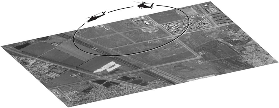
The simulation environment

The flowchart of the simulation is shown in Figure 5. At first, a trajectory is designed as the input into a navigation state generator. The outputs of the generator, such as velocity and attitude, are used to obtain a sub-image from the whole map at this moment. Then features are detected and matched with those in the last simulated image and the corresponding features are used to estimate the homography robustly. The motion of the vehicle is estimated with the homography and the relative distance provided by the state generator. Finally, the visual measurement is fused with the inertial output, which is also simulated by the navigation state generator, by the delay-based EKF. The output of the navigation is compared with the original result provided by the navigation state generator.

Figure 5.

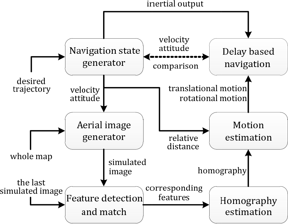
The simulation flowchart

The parameters of the sensors are simulated according to the characteristics of the real ones in the experiment. The uncertainty of the image is one pixel. The noise intensity of the gyroscopes is set 0.3% with the bias of 0.3%. The noise intensity of the accelerometers is 0.1m/s² with a bias of 0.3m/s². The measurement is obtained by the homography decomposition and the conversion from the camera coordinate to the navigation coordinate, which is a rather complex process. Therefore in this paper, the measurement covariance is determined by a statistic approach in the simulation. Suppose that the state of the small UAV (position, velocity and attitude) was estimated accurately at an instant, the state at the next instant can be obtained by both the state generator, as shown in Figure 5 and the visual measurement from the decomposition of the calibrated homography can be calculated from consecutive images. The difference between these two methods is recorded and this process is repeated many times at different positions, velocities or attitude. The data are used for the determination of the variance for each item in the measurement vector. The measurement covariance is set as R₁ = diag(3,3,3,2,2,2,2) and R₂ = diag(3,3,3) in the simulation. For the real experiment, the measurement covariance is first set to be the same as the simulation. After the real flight, the acquired sensor data are analysed offline and the measurement covariance is optimized to get a better performance from the filter.

The initialization of the bias in the inertial sensors is another important element in the filter. In the simulation, the biases are initialized by the following approach. The UAV is put on the ground without any movement. The visual measurement is replaced by information on the changeless position, zero velocity and changeless attitude. Then, after a few seconds, the bias of the inertial sensors will be well estimated. Figure 6 and 7 show the initialized process of the three-axis gyroscopes and the three-axis accelerometers. Both these kinds of bias can be initialized accurately.

Figure 6.

The initialization of the bias of the gyroscopes

Figure 7.

The initialization of the bias of the accelerometers

4.2 The effect of the measurement delay on the filter

Firstly, the effect of the measurement delay on the EKF filter is analysed. In this filter, the attitude estimated by the camera is a real-time measurement, while the velocity measurement is set with a different delay, from 0 to 2 seconds with an interval of 0.2 seconds. The ratio of the standard deviation of the velocity estimate after the stabilization is calculated for the analysis of the delay effect on the filter. The ratio is defined as r(t) = std(t)/std(0), where std(t) is the standard deviation with a delay of t seconds and r(0) = 1. The simulation runs several times at each delay step and the average is taken as the final result.

Figure 8 shows the delay effect on the velocity estimation. It can be seen that the standard deviations of vx and vy increase linearly with the measurement delay. When the delay reaches 2 seconds, the standard deviation is about four times larger than that estimated by the non-delayed measurement. Our on-board avionics run at about 2Hz for the visual measurement. It can be concluded from this figure that a measurement delay of 0.5 seconds results in an increase in the standard deviation of about 50%. The delay of the visual measurement has a non-negligible effect on the estimate accuracy of the filter. The delay effect on the estimate of the velocity in the down direction is not as evident as others. One reason is that vz does not change as much in the desired trajectory, compared with the velocities in the horizontal directions. Hence, there is no clear difference between the delayed and non-delayed measurements.

Figure 8.

The delay effect on the velocity estimation

4.3 The effect of the time interval of the visual process

In the velocity measurement update, the time interval t_m between two visual processes is considered as an important factor to the filter. The frequency of the measurement updates is determined by the time interval. For example, if t_m = 0.5 seconds, the measurement update runs at 2Hz. Moreover, the time interval affects the assumption in Equation (26). If t_m is too long, this assumption might be invalid. So another simulation is carried out to test the effect of the time interval. Two kinds of measurements are simulated: one is the velocity generated under the assumption at Equation (26); another is the “real” instantaneous velocity. The output of the system is defined as r(t) = std_a(t)/std_r(t), where std_a(t) and std_r(t) are the standard deviations of the velocity estimates of the above two kinds respectively, with t as the time interval.

The effect of the time interval on the velocity estimation is shown in Figure 9. The time interval changes from 0.1 to 1.9 seconds, but the standard deviation does not increase accordingly. The biggest is only 1.24 times the referential, when t_m equals 1.7 seconds. The time interval has some effect on the filter by the frequency of the measurement update. However, the velocity estimate is stable in spite of the change in the time interval. This means that the assumption is reasonable in this application and the velocity calculated by our proposed method can be used in the measurement update of the filter.

Figure 9.

The effect of the time interval

4.4 Comparison with the augmented navigation

The last simulation test is about the comparison of the proposed navigation and the general augmented system. Both of them take the homography-based method, which is described in Section 2, to obtain the visual measurement. In the augmented filter, the state is expanded by including the state of the vehicle when the previous visual measurement is calculated. The augmented EKF is built mainly according to [17]. Matrix partition is applied for the optimization of the augmented filter calculation.

The error comparisons of the attitude and the velocity are shown in Figure 10 and Figure 11, respectively. Both the methods can limit the attitude and velocity errors within (–1°, 1°) and (–1m/s, 1m/s). They have similar performances after the filters are stable. Figure 12 shows the comparison of the position error. The lines labelled “integrated” are the differences between the real position and the position calculated by the estimated velocity integration of the proposed filter. The correction of the proposed filter can be seen by comparing it with the integrated. The error of the position estimate of the proposed method is generally smaller than that of the velocity integration. Some drift is expected in the position estimation by these mapless methods. However, the drift has been remarkably reduced compared to approaches using inertial sensors alone.

Figure 10.

The comparison of the attitude errors in simulation

Figure 11.

The comparison of the velocity errors in simulation

Figure 12.

The comparison of the position errors in simulation

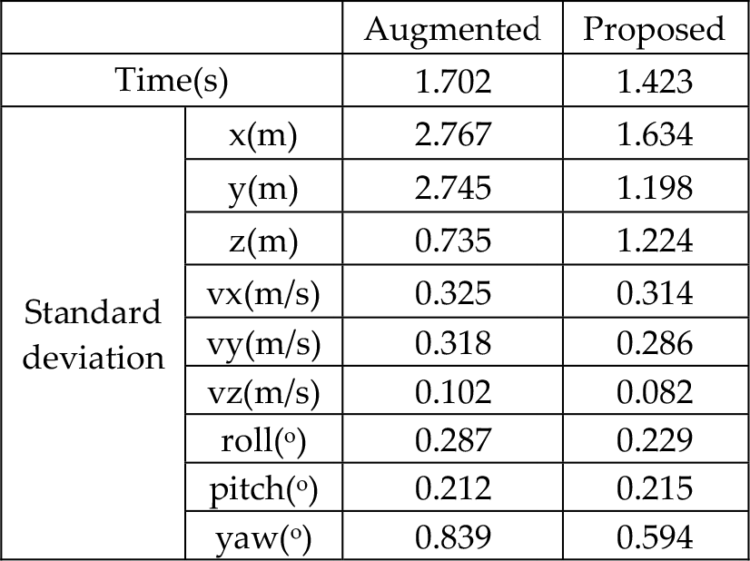
The comparison of the standard deviations, which is shown in Table 1, also verifies the above conclusion. In general, the proposed delay-based navigation system has almost the same performance as the augmented system in estimate accuracy. The average computing time is also recorded in Table 1. In the simualtion, these methods are realized by Matlab on a laptop (Window7 32-bit, Intel(R) Core(TM) i7-2670QM, 2.20GHz, 4GB RAM). Since the image processing is completed in advance, the recorded time is only for the whole process of the filter (6187 loops for the state propagation). Despite the fact that the matrix partition is applied, the average computing time of the augmented method is still about 1.702 seconds. The proposed method requires only 1.423 seconds for the whole calculation. This means that our method can reduce the computational complexity by about 20%, while keeping almost the same performance as the augmented approach.

Table 1.

The comparison of two navigation systems

		Augmented	Proposed
Time(s)		1.702	1.423
Standard deviation	x(m)	2.767	1.634
	y(m)	2.745	1.198
	z(m)	0.735	1.224
	vx(m/s)	0.325	0.314
	vy(m/s)	0.318	0.286
	vz(m/s)	0.102	0.082
	roll(°)	0.287	0.229
	pitch(°)	0.212	0.215
	yaw(°)	0.839	0.594

5. Experiments

5.1 System description

The experimental test bed helicopter is shown in Figure 13. The on-board avionics includes an Rt20 differential GPS receiver, an ADIS16355 IMU, an MS5540 barometric altimeter, a three-axis magnetometer that is composed of HMC1052 and HMC1041, an MV-1300UC colour industrial digital camera and four on-board computers. DSP TI28335 runs the navigation filter and fuses the measurements of GPS, IMU and other sensors. ARM LPC1766 is equipped to guide and control the small UAV. FPGA EP2C is in charge of the flight data recording and the control switch between a human pilot and autopilot. PC-104 PCM3362 is used as the vision computer to receive the sensor data from the FPGA and record the aerial images simultaneously. The on-board equipment is shown in Figure 14.

Figure 13.

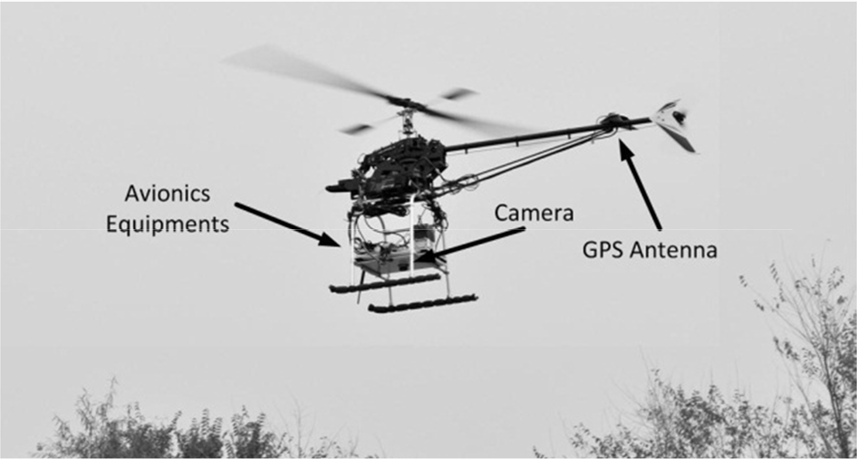
The experimental helicopter test bed

Figure 14.

The on-board avionics

The proposed visual navigation system consists of three main parts: image processing, homography-based motion estimation and sensor fusion. Figure 15 shows a flowchart of the whole system. In image processing, SIFT is applied to detect the features from consecutive frames, with a fuzzy controller to adjust the threshold online. Then the motion of the vehicle is estimated by a homography model of corresponding features. Afterwards, the motion is transferred into the attitude and velocity of the vehicle and fused with the inertial estimation by an indirect EKF with a delay-based measurement update.

Figure 15.

The system flowchart

5.2 Test of the vision-aided inertial navigation system

An experiment is carried out to test the performance of the proposed navigation system with the above test bed. A flat wasteland is chosen as the experimental field. The relative height, which is used to recover the translational motion of the vehicle, is estimated by the output of the barometric sensor compensated by the initial height measurement on the ground. This measurement method is reasonable since the image scene is supposed to be a ground plane during the flight. The relative height can also be measured by adding other sensors, such as ultrasonic or laser rangefinders. However, the discussion of the relative distance estimate methods is not the focus of this paper. During the experiment, a skilled human pilot operates the helicopter manually. The sensor data are recorded on-board and analysed offline. The data is acquired at a rate of 50Hz for the inertial sensors and 2Hz for the visual sensor. The performance of the proposed Vision/INS navigation system is evaluated by comparing it with the augmented and referential GPS/INS navigation.

The attitude comparison of the whole flight is shown in Figure 16. The visual measurement does not work during the take-off and landing, in which periods the visual estimation is not accurate enough due to the rapid change of the aerial images. Thus, the visual measurement takes effect from the 16th second to 107th second in this figure. The GPS signal is cut off when the visual measurement is available. The augmented filter is also included in this comparison. The error here means the difference between the estimate and the output of the GPS/INS navigation. Figure 17 and 18 illustrate the comparisons of velocity and position estimates in the navigation coordinates.

Figure 16.

The comparison of the attitude errors in experiment

Figure 17.

The comparison of the velocity errors in experiment

Figure 18.

The comparison of the position errors in experiment

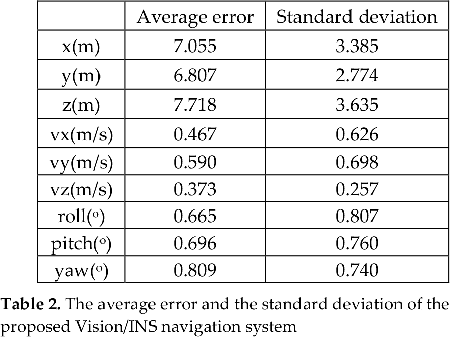
The effectiveness of the proposed Vision/INS method has been verified by this experiment. In the proposed system, the visual measurement is applied to fuse with the inertial sensors for the state estimation of the vehicle when GPS is unavailable. This filter is able to provide stable and reliable estimates of the attitude and velocity with high accuracy, while the position estimate is subject to drift. This is a well-known drawback for any mapless method. In this filter, the drift has been greatly limited by the visual measurement. The average error and standard deviation of the proposed method are shown in Table 2.

Table 2.

The average error and the standard deviation of the proposed Vision/INS navigation system

	Average error	Standard deviation
x(m)	7.055	3.385
y(m)	6.807	2.774
z(m)	7.718	3.635
vx(m/s)	0.467	0.626
vy(m/s)	0.590	0.698
vz(m/s)	0.373	0.257
roll(°)	0.665	0.807
pitch(°)	0.696	0.760
yaw(°)	0.809	0.740

6. Conclusion and future work

This paper presented a vision-aided inertial navigation system for small UAVs in GPS-denied environments. A delay-based measurement update method was proposed to introduce the homography-based visual measurement into the indirect EKF without any state augmentation. The effects of the delay measurement and the time interval of the visual process on the filter have been analysed by simulations. The simulation results indicated that the proposed delay-based method can reduce the computational complexity by about 20%, compared with the general augmented filter, with almost the same estimate accuracies. The effectiveness of the proposed method has been verified by an experiment. The navigation system developed in this paper achieves its good performance by comparing with the referential GPS/INS navigation for small UAVs. In summary, the proposed vision-aided inertial navigation method can provide a reliable state estimate for small UAVs in GPS-denied environments.

Future work will be carried out in two aspects. Firstly, other sensors will be added to measure the relative distance more precisely. Secondly, as well as the attitude and the velocity, the position of the vehicle can also be estimated by the proposed navigation but suffers a drift. This drift is mainly due to the accumulation of the error from the velocity estimation. Additional observations are required if the full autonomy of the UAV in GPS-denied environment is considered. In the future, a monocular SLAM system will be developed based on this system to improve the position estimation and the autonomy of small UAVs.