Sage Journals: Discover world-class research

Abstract

The formation task achieved by multiple robots is a tough issue in practice, because of the limitations of the sensing abilities and communicating functions among them. This paper investigates the decentralized formation control in case of parameter uncertainties, bounded disturbances, and variant interactions among robots. To design decentralized controller, a formation description is firstly proposed, which consists of two aspects in terms of formation pattern and interaction topology. Then the formation control using adaptive neural network (ANN) is proposed based on the relative error derived from formation description. From the analysis on stability of the formation control under invariant/variant formation pattern and interaction topology, it is concluded that if formation pattern is of class C^k, k ≥1, and interaction graph is connected and changed with finite times, the convergence of the formation control is guaranteed, so that robots must form the formation described by the formation pattern.

Keywords

adapted neural network control interaction topology Lyapunov theorem for nonsmooth systems switched system

1. Introduction

Multiple robots coordination to form a kind of pattern is an interesting phenomenon, which also has wide applications in highway transportation, army inspection, and external stars exploration. If a predetermined formation pattern is given, a group of robots forming formation will be investigated in this paper.

Formation is viewed as a kind of information consensus in which robots or agents interact with each other using various sensors and communication techniques. For example, a simple discrete-time Vicsek model is built up, which commands a group of robots to move on the plane with the same heading (Vicsek, T., Czirok, A., Jacob, E. B. & Schochet, O., 1995). Using graph theory, the theoretical explanation about Vicsek model and its extended version are provided in (Jababaie, A., Lin, J. & Morse, A. S., 2003) and (Ren, W. & Beard, R. W., 2005).

In robotic applications, there are several approaches to multiagent coordination referred in the literature, namely leader-following, behavioral, potential fields, virtual structures, and generalized coordinates.

In leader-following, one of the agents is designated as the leader, which tracks predefined reference trajectories, with the rest of the members designated as followers which follow the leader or their neighbors (Wang, P. K. C., 1991, Sugar, T. & Kumar, V., 1998, Desai, J. P., Ostrowski, J. & Kumar, V., 1998). Leader-following paradigm is easy to understand and implement. In addition, the formation can still be maintained even if the leader is perturbed by some disturbances. However there is no explicit feedback to the formation.

The virtual structure approach is another technique widely used in formation control, where the entire formation is treated as a single structure (Lewis, M. A. & Tan, K.H., 1997, Moscovitz, Y. & DeClaris, N., 1998, Tan, K.H. & Lewis, M.A., 1996). Using virtual structure approach, it is easy to prescribe a coordinated behavior for the group. And feedback to the virtual structure is naturally defined. Hence even if some agents are failed, the formation is still maintained. However this approach is not proper when formation is time-varying or needs to be frequently reconfigured.

A general approach is developed to model and control of formations in terms of generalized coordinates (Spry, S. C., 2002, Spry, S. & Hedrick, J. K., 2004). It produces asymptotic tracking of trajectories, including those with time-varying rotations and shape, and allows the controller to be formulated in terms of quantities which are closely related to the performance objectives of tracking a group trajectory while maintaining a desired formation shape.

All three techniques mentioned above require that the full state of the leader or virtual structure be communicated to each member of the formation. In contrast, behavior-based approach is decentralized and may be implemented with less communication. The basic idea of the behavioral approach is to prescribe several desired behaviors for each agent, such as target seeking, collision/obstacle avoidance, and interaction with neighbors, so that desirable group behavior emerges finally (Jonathan, R. T., Beard, R. W. & Young, B. J., 2003, Balch, T. & Arkin, R. C., 1998, Chen, Q. & Luh, J. Y. S., 1994). As a decentralized implementation, behavioral approach enables agents derive controls for multiple competing objectives simultaneously. In addition, there is explicit feedback to the formation. The primary shortage is that group behavior cannot be explicitly defined. Hence it is difficult to analyze group behavior mathematically.

Another decentralized approach of formation control is potential fields approach (Schneider, F. E. & Wildermuth, D., 2003). In this method, different virtual forces belonging to robots, obstacles and the desired shape of formation are combined and used to move each robot to its desired position inside the formation. Similar to behavioral approach, the control derived based on several forces enables agents form a formation, while avoiding collision with obstacles or others. But the formation pattern (shape) needs to be broadcasted to all members. Hence comparing with behavioral method, it needs more communication cost. Moreover, for mobile robots with nonholonomic constraints, it is difficult to provide a mechanism to solve special movements induced by nonholonomic constraints.

Just as mentioned, leader-follower approach is easily implemented in practice. Comparing with virtual structure approach, leader-follower paradigm can realize time-varying formation pattern. Even under complex conditions, such as uncertain parameters and unknown disturbances, individual control in leader-following paradigm can guarantee formation stability. Hence it is easily realized in practical applications than generalized coordinates. Comparing with behavioral approaches, the feasibility of leader-following paradigm can be guaranteed mathematically. Therefore in this paper, we adopt leader-follower to realize formation in which information exchange is directed, and robots are required to form formation according to certain formation patterns. The major problem is to develop a decentralized control strategy to guarantee formation's stability.

To describe formation behavior in the continuous-time case, a technique of leader-to-formation stability (LFS) is proposed in which formation stability is analyzed by input-to-state stability method (Tanner, H. G., Pappas, G. J. & Kumar, V., 2004). Another important technique broadly used for formation control stability is Lyapunov theory (Liu, Y., Passino, K. M. & Polycarpou, M., 2001, Ogren, P., Egerstedt, M. & Hu, X., 2002, Kowalczky, W. & Kozlowski, K., 2004, Bicho, E. & Monteiro, S., 2003, Balch, T. & Hybinette, M., 2000).

Since in practical situations, most platforms of formation are constructed using multiple nonholonomic mobile robots which are always modeled with some uncertain parameters, and because of limitations on sensors and communication ability, relationship among robots described by formation patterns and interaction topology is always variant, the linear feedback-control law proposed in (Tanner, H. G., Pappas, G. J. & Kumar, V., 2004) can not be employed for the formation. Hence we extend the ANN control designed for smooth continuous system (Fierro, R. & Lewis, F. L., 1998, Lewis, F. L., Yegildirek, A. & Liu, K., 1996) to the case of nonsmooth, even noncontinuous systems, so that the control strategy is able to make robots keep in regular formation in practical environment.

The rest of this paper is organized as follows. In Section 2, we introduce the description about formation structure using graph theory. Based on the description, Section 3 presents the sufficient condition of formation control in terms of a Lemma. Section 4 introduces the decentralized control strategy using adaptive neural network. Three theorems are presented in Section 5 to investigate the feasibility of this formation control under different conditions, including variant or invariant formation pattern and interaction topology. The feasibility is validated by a simulation, and some discussions about practical applications are provided. Finally conclusions are drawn in Section 6.

2. Description of Formation's Internal Information

In this paper, a group of robots are labeled by R_i (i = 1, …, N), where R_l represents the leader of the formation. Let P^d = [p₁^d p₂^d … p_N^d]^T denote the desired positions of all robots relative to robot l. Obviously, p_l^d = 0. Let P = [p₁ p₂ − p_N]^T denote the coordinates of robots in universal frame. The internal information of a formation consists of two aspects.

(1) Formation pattern (denoted by D^d (t)

Formation pattern describes the desired formation shape by a matrix, D^d = {D_ij^d}_NxN, whose elements present all desired relative distances between the robots, i.e., D_ij^d = p_i^d − p_j^d. Obviously D_ii^d = 0. Moreover we denote D^d(t) as the time-varying formation pattern. We also let D = {D_ij}_NxN denote real relative distances between robots, where D_ij = p_i − p_j. Fig. 1 shows an example of relative matrix D^d. In the example, R₁ is assigned to play the role of the formation leader.

Fig. 1.

A formation pattern including six robots. Only the x-axis coordinate of D^d is displayed below the figure

(2) Interaction topology (denoted by G)

To detect the relative positions within a formation, robots need to make contacts with each other. Hence it needs to describe interactions among robots. No matter what technique is applied to realize interaction, we use graph theory to present interactions among robots.

A directed graph G is exploited to describe the interaction topology of formation, which consists of a set of vertices (robots) Ξ and a set of arcs Ω, where α = (v, w) ∈ Ω and v, w ∈ Ξ. Arc α(v, w) represents that R_v takes R_w as a reference object to compute its desired reference position. Since a robot may interact with several robots simultaneously, its reference position may be determined by several robots. Let G = {g_ij}_NxN denote adjacency matrix associated with graph G, where g_ij represents a kind of weight denoting the degree of R_j affecting the reference position of R_i. G has a property,

\sum_{j = 1}^{N} g_{i j} = 1 .

(1)

And we define H = {h_ij}_N×N as H = I − G. Due to the property of G, it holds that $\sum_{j = i}^{N} h_{i j} = 0$ .

An example of interaction topology and adjacency matrix is illustrated in Fig. 2. Since R₁ plays the role of the leader, it holds that g₁₁ = 1, while other diagonal entries are zero g_ii = 0, (i = 2, …, N)).

Fig. 2.

An example of interaction topology among six robots, where L_max represents the maximal range of interaction, so that a robot can make contact with other robots within this range

Obviously combining these two aspects, the internal information of a formation can be described by G o D^d, where the operator o means Hadamard product (to simplify denotation, we let D^d denote both time-fixed and time-varying formation patterns).

3. Motivation of Formation Control

Based on the description of formation, let E = {e_j}_N×1 = (G o D − G o D^d)1_N×1 be a relative error vector, so that it follows that

E = H P - G \circ D^{d} 1_{N \times 1} = P - (G P + G \circ D^{d} 1_{N \times 1})

(2)

Since R_l plays the role of the formation leader, it holds g_ll = 1, while g_lj = 0, j = 1, …, N, and j ≠ l. Therefore the l th element of the relative error, e_l, equals zero. It's reasonable because the adjacency graph is built relative to the leader, the relative error of R_l should be zero.

The following lemma is introduced.

Lemma 1. Given an error shown in (2), if the adjacency matrix G is connected, when E = 0, all robots will follow the leader of the formation and form a formation described by D^d (or D^d(t)).

Proof: See Appendix A.1.

Lemma 1 suggests a way to realize formation control. Since GP + G o D^d1_N×1 in (2) can be measured on real time, if G and D^d are known for all members of the formation, every robot can control itself to follow a reference point determined by GP + G o D^d 1_N×1 in order to form formation.

4. Individual Control Strategy

4.1. Dynamic Description of Individual Robot

A kind of two-wheel car-like mobile robot shown in Fig. 3 is employed to realize formation. The dynamics of robot is expressed as

Fig. 3.

A two-wheel-driven mobile robot.

M (q) \overset{..}{q} + V (q, \dot{q}) \dot{q} + τ_{d} = J^{T} (q) λ + B (q) τ,

(3)

where q = [p_x p_y θ]^T represents general coordinate, τ_d represents bounded disturbance and unmodeled dynamics. We take the center of mass as the robot's position. Matrices referred in the equation are given by

\begin{array}{l} M (q) = [\begin{matrix} m & 0 & m d sin θ \\ 0 & m & - m d cos θ \\ m d sin θ & - m d cos θ & I_{0} + m d^{2} \end{matrix}], \\ τ = {[τ_{1}, τ_{r}]}^{T} V (q, \dot{q}) = [\begin{matrix} 0 & 0 & m d \dot{θ} cos θ \\ 0 & 0 & m d \dot{θ} sin θ \\ 0 & 0 & 0 \end{matrix}], \\ B = \frac{1}{r} [\begin{matrix} cos θ & cos θ \\ sin θ & sin θ \\ L & - L \end{matrix}], J (q) = [sin θ - cos θ d] . \end{array}

Normally the nonholonomic constraints can be expressed as $J (q) \dot{q} = 0 or {\dot{p}}_{x} sin θ - {\dot{p}}_{y} cos θ + d \dot{θ} = 0$ . Then the second order derivative of θ is expressed as:

\begin{array}{l} \overset{..}{θ} = \frac{1}{d} ({\overset{..}{p}}_{y} cos θ - {\overset{..}{p}}_{x} sin θ) \\ + \frac{1}{2 d^{2}} ({\dot{p}}_{x}^{2} - {\dot{p}}_{y}^{2}) sin 2 θ - \frac{1}{d^{2}} {\dot{p}}_{x} - {\dot{p}}_{y} (c o s^{2} θ - {sin}^{2} θ) . \end{array}

(4)

It is easy to find a full rank matrix A(q) which is formed by the vectors spanning the null space of constraint matrix J(q) such that A^T (q)J^T (q) = 0, where $A (q) = [\begin{matrix} cos θ & - d sin θ \\ sin θ & d cos θ \\ 0 & 1 \end{matrix}]$ . Multiplying both sides of (3) with A^T to eliminate nonholonomic constraint forces λ, it follows that

A^{T} M (q) \overset{..}{q} + A^{T} V (q, \dot{q}) \dot{q} + {\bar{τ}}_{d} = A^{T} B (q) τ,

(5)

where ${\bar{τ}}_{d} = A^{T} τ_{d}$ . If define p = [p_x p_y]^T, $T = [\begin{matrix} cos θ & sin θ \\ - sin θ & cos θ \end{matrix}]$ and $M_{c} = [\begin{matrix} m & 0 \\ 0 & \frac{I}{d} \end{matrix}]$ , (5) can be transformed to

M_{c} T \dot{p} + M_{c} T \dot{p} = A^{T} B τ - {\bar{τ}}_{d} .

(6)

4.2. Neural Network Controller

Following (2), we take GP + G o D^d1_N×1 as local desired position for individual control design. If we decompose GP + G o D^d1_Nx1 for individual robots, the desired reference point for R_i is of the form $p_{i}^{d} = \sum_{j = 1}^{N} g_{i j} (p_{j} + D_{i j}^{d})$ Therefore we define the individual relative position error as

e_{i} = p_{i} - p_{i}^{d} = p_{i} - \sum_{j = 1}^{N} g_{i j} (p_{j} + D_{i j}^{d}) .

(7)

A filtered error is defined as z_i = ė_i + Λe_i. If define a temporal variable, ṗ_i^r = ṗ_i^d − Λe_i, then z_i = ṗ_i − ṗ_i^r. Substitute it into (6), and let z˜_i = T_iz_i, thus

\begin{matrix} M_{c} {\tilde{z}}_{i} = A^{T} B τ_{i} - {\bar{M}}_{i} {\overset{..}{p}}_{i}^{r} - {\bar{V}}_{i} {\dot{p}}_{i}^{r} - {\bar{τ}}_{i d} . \\ w h e r e {\bar{M}}_{i} = [\begin{matrix} m_{i} & 0 \\ 0 & \frac{I_{i}}{d_{i}} \end{matrix}] [\begin{matrix} cos θ_{i} & sin θ_{i} \\ - sin θ_{i} & cos θ_{i} \end{matrix}], \\ {\bar{V}}_{i} = \frac{I_{i}}{d_{i}} (\dot{x} sin θ_{i} - \dot{y} cos θ_{i}) [\begin{matrix} m_{i} & 0 \\ 0 & \frac{I_{i}}{d_{i}} \end{matrix}] [\begin{matrix} sin θ_{i} & - cos θ_{i} \\ cos θ_{i} & sin θ_{i} \end{matrix}] . \end{matrix}

(8)

Because there may exist parameter uncertainties, we use a neural network to model ${\bar{M}}_{i} {\overset{..}{p}}_{i}^{r} + {\bar{V}}_{i} {\dot{p}}_{i}^{r}$ on-line.

A nonlinear function $f (X_{i}) = {\bar{M}}_{i} {\overset{..}{p}}_{i}^{r} + {\bar{V}}_{i} {\dot{p}}_{i}^{r}$ is defined in which $X_{i} = [{\dot{p}}_{i} sin θ_{i} cos θ_{i} {\overset{..}{p}}_{i}^{r} {\dot{p}}_{i}^{r}]^{T}$ . To simplify the expression, the subscript i is omitted. We suppose that there exists a two-layer feedforward NN like Fig. 4 shows which can approximate f(X), i.e.

Fig. 4.

A two-layer feedforward neural network

f (X) = W^{T} σ (V^{T} X) + ɛ,

(9)

where V ∈ R^N_I×N_H represent the input-to-hidden-layer interconnection weights, W ∈ R^N_H×N_O represent the hidden-layer-to-outputs interconnection weights, where N_H, N_I and N_O are the numbers of neurons in the hidden layer, the input layer, and the output layer respectively, the activation function σ(·) is in the form of $σ (x) = \frac{1}{1 + e^{- x}}$ , ε is the NN functional approximation error.

Let Y_M denote the bound of ideal weights, such that ‖W‖_F + ‖V‖_F ≤ Y_M.

Firstly, there is a property about the bounding fact.

Property 1: X is bounded by

‖ X ‖ \leq c_{1} Φ + c_{2} ‖ \tilde{z} ‖ + c_{3},

(10)

where c₁ to c₃ are positive scalars, Φ is the bound which will satisfy

‖ \begin{matrix} p^{d} \\ {\dot{p}}^{d} \\ {\overset{..}{p}}^{d} \end{matrix} ‖ \leq Φ .

(11)

Proof: See Appendix A2.

The purpose of NN learning is to construct a NN function f̂(X) to estimate f(X) on-line, which can be written as

\hat{f} (X) = {\hat{W}}^{T} σ ({\hat{V}}^{T} X),

(12)

where Ŵ and V̂ are estimates of NN weights.

The estimated errors are defined as f˜ = f − f̂, W˜ = W − Ŵ, and V˜ = V − V̂. And the hidden-layer output error is defined as $\tilde{σ} = σ - \hat{σ} = σ (V^{T} X) - σ ({\hat{V}}^{T} X)$ .

Applying Taylor series expansion, we can obtain

σ (V^{T} X) = σ ({\hat{V}}^{T} X) + σ' ({\hat{V}}^{T} X) {\tilde{V}}^{T} X + O ({\tilde{V}}^{T} X)^{2},

(13)

where ${σ^{'} (\hat{y}) = \frac{\partial σ (y)}{\partial y} ∣}_{y = \hat{y}}$ . Therefore,

\tilde{σ} = σ' ({\hat{V}}^{T} X) {\tilde{V}}^{T} X + O ({\tilde{V}}^{T} X)^{2},

(14)

where $O ({\tilde{V}}^{T} X)^{2}$ satisfies the following property.

Property 2:

‖ O {({\tilde{V}}^{T} X)}^{2} ‖ \leq C_{4} + C_{8} {‖ \tilde{V} ‖}_{F} ‖ \tilde{z} ‖ + c_{9} {‖ \tilde{V} ‖}_{F} .

(15)

where c₄, c₈, and c₉ are positive scalars.

Proof: See Appendix A.3.

Substituting f(X) into (8), we have

M_{c} \dot{\tilde{z}} = A^{T} B τ - f (X) - {\bar{τ}}_{d} = A^{T} B τ - W^{T} σ (V^{T} X) - {\bar{τ}}_{d} + ɛ .

(16)

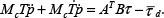
Now we design the input-output feedback linearization controller in terms of (17) and the adaptive backpropagation learning algorithm in terms of (18) respectively. Consequently the architecture of formation control is shown in Fig. 5.

Fig. 5.

The architecture of formation control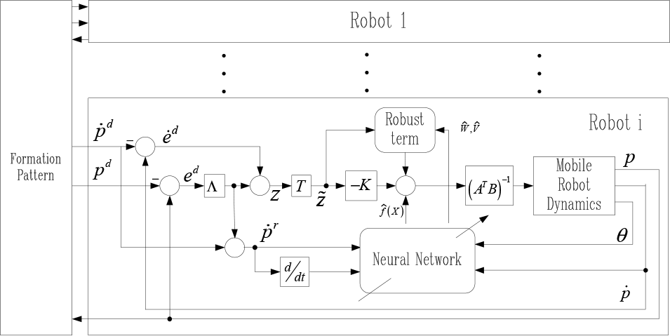

τ = (A^{T} B)^{- 1} ({\hat{W}}^{T} σ ({\hat{V}}^{T} X) - K \tilde{z} + γ),

(17)

\begin{array}{l} \dot{\hat{W}} = F \hat{σ}' {\hat{V}}^{T} X {\tilde{z}}^{T} - F \hat{σ} {\tilde{z}}^{T} - κ F ‖ \tilde{z} ‖ \hat{W}, \\ \dot{\hat{V}} = - U X {(\hat{σ}'^{T} \hat{W} \tilde{z})}^{T} - κ U ‖ \tilde{z} ‖ \hat{V}, \end{array}

(18)

where K = diag{k₁, k₂} in which k₁ and k₂ are positive scalars, γ is a robust control term to suppress the disturbance of unmodeled structure of dynamics τ_d and functional approximation error of NN ε, F and U are positive definite design parameter matrices governing the speed of learning.

Substitute the control law into (16), and let σ and $\hat{σ}$ denote σ(V^TX) and $σ ({\hat{V}}^{T} X)$ respectively, thus

M_{c} \dot{\tilde{z}} = - K \tilde{z} - W^{T} σ + {\hat{W}}^{T} \hat{σ} + γ - {\bar{τ}}_{d} + ɛ .

(19)

Adding and subtracting $W^{T} \hat{σ}$ and ${\hat{W}}^{T} \tilde{σ}$ , and using (13) and (14), we have

M_{c} \dot{\tilde{z}} = - K \tilde{z} - {\tilde{W}}^{T} (\hat{σ} - \hat{σ}' {\hat{V}}^{T} X) - {\hat{W}}^{T} \hat{σ}' {\tilde{V}}^{T} X + s + γ,

(20)

where s(t) is a disturbance term,

s (t) = - {\tilde{W}}^{T} \hat{σ}' V^{T} X - W^{T} O ({\tilde{V}}^{T} X) - {\bar{τ}}_{d} + ɛ .

(21)

5. Stability on Formation Control

In Section 2, it is mentioned that there are two aspects, the formation pattern D^d and interaction matrix G, describing the information within a formation. In practice, due to the different requirements about formation tasks, formation pattern and interaction topology may be invariant or variant respectively. In this section, the stability of the formation control under three different situations covering all possible kinds of formation pattern and interaction topology will be analyzed.

5.1. Stability under Invariant Formation Pattern and Invariant Interaction Topology

The words “invariant formation pattern” in the title means that during the process, the formation pattern D^d is constant, or the desired formation shape is static. The following theorem describes the convergence of formation control with fixed formation pattern.

Theorem 1: Assume that for a multi-robot system designed for formation task with a predetermined leader, formation pattern is fixed, and adjacency matrix associated with interaction graph is strong connected and invariant. If there are bounded disturbance and parameter uncertainty about robot structure, the robots must form a formation using individual control strategy represented in (17) and (18).

Proof: See Appendix A.4.

Remark 1: It should be mentioned that the proof of convergence does not assert that the weight error Ŵ and V̂ will converge to zero. That means although f̂(X) approaches to f(X), the Ŵ and V̂ may not converge to the desired weights W and V without error eventually. But since for a formation task, the most important thing is to keep a formation shape, it is acceptable that there exist estimated errors on NN weights.

The simulation of a formation with fixed formation pattern is proposed, where six robots are required to form a hexagon formation. The size of robot is 0.14 × 0.08m, while its weight is 1kg. The NN used in individual control includes a hidden layer with 40 nodes. All weights of NN are initialized as random values within [0,1]. R₁ plays the role of formation leader, which is required to follow a trajectory expressed as p_y^d = 0.3sin(p_x^dπ). The simulation results are shown in Fig. 6. From Fig. 6 (a), we observe that six robots scattering randomly at the beginning can form a formation. The invariant interaction topology is denoted by arrows shown in the figure (a). And Fig. 6 (b) shows the relative errors of robots, where e_x and e_y mean the relative errors in X-axis and Y-axis directions respectively. Obviously all errors converge to zero in the end. So the individual control strategy works very well.

Fig. 6.

Simulation results of fixed formation pattern and interaction topology

5.2. Stability under Variant Formation Patterns and Invariant Interaction Topology

The variant formation pattern means that the formation pattern is changed over time. Just as mentioned in Section 2, the time-varying formation pattern is denoted by D^d (t).

5.2.1. The Problem Induced by Variant Formation Pattern

In practice, due to moving obstacles, perceiving limits, and even direct control commands, formation pattern should be changed on real time. For example, when a formation is passing through an obstacle field, if the formation perceives an obstacle which is on the way of its members, it has to generate another formation pattern so that its members can avoid the obstacle according to the new formation pattern. A simple illustration about the change of formation pattern is shown in Fig. 7 where there are two robots forming a leader-follower formation. When it is perceived that the obstacle is on the way of R₂, R₂ has to change its relative position from parallel to R₁ to behind R₁. Hence a transition process, which is between the dashed verticals in Fig. 7, is necessary to make formation pattern change continuously. It is obvious that since the formation pattern is changed on real time, D^d(t) over the whole process must be not of class C^∞, i.e., D^d(t) doesn't have continuous derivatives of any order, so that we can not guarantee the convergence of formation control using Theorem 1. To ensure convergence of the formation control, we have to figure out the conditions under which the adaptive NN control can be applied. Theorem 2 presents the conditions which ensure stability of formation control.

Fig. 7.

An example of variant formation pattern

5.2.2. Convergence of Formation Control with Variant Formation Pattern

Theorem 2: If all assumptions are the same as Theorem 1 except that formation pattern is time-varying and D^d(t) is of class C^k, k ≥ 1, the robots must converge to the formation pattern using individual control strategy represented in (17) and (18).

Proof: See Appendix A.5.

From Theorem 2, it is concluded that the sufficient condition of convergence of the formation with invariant interaction topology is that the formation pattern is at least of class C¹ continuous.

Remark 2: Now we can propose a practical strategy to generate a transition process in order to make formation pattern be of class C¹.

Assume that within the duration of [t₁, t₂], formation pattern is required to change from D₁^d(t) to D₂^d(t), which is of class C^∞ respectively. The transition process is defined as

ψ (t) = η (t) D_{1}^{d} (t) + (1 - η (t)) D_{2}^{d} (t) .

(22)

where t ∈ [t₁, t₂], η(t) is a function which satisfies the following boundary conditions.

{η (t_{1}) = 1, η (t_{2}) = 0, \frac{d η (t)}{d t} ∣}_{t = t_{1}} {= \frac{d η (t)}{d t} ∣}_{t = t_{2}} = 0,

(23)

Applying the transition process ψ(t), it is easy to prove that the formation pattern D^d(t) described in (24) is of class C¹.

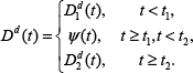
D^{d} (t) = {\begin{matrix} D_{1}^{d} (t), & t < t_{1}, \\ ψ (t), & t \geq t_{1}, t < t_{2}, \\ D_{2}^{d} (t), & t \geq t_{2} . \end{matrix}

(24)

Hence such a general transition process ensures that the pattern satisfies the conditions in Theorem 2, so that the formation must be constructed. The simulation proposed in the next subsection includes an example of such transition process.

5.3. Stability under Variant Interaction Topology

5.3.1. Noncontinuous System Resulting from Variant Interaction Topology

Since interaction is affected by the robot's ability such as perceiving range and communication bandwidth, one robot is able to make contact with other robots within its perceiving range. If the distance between robots become too far to set up interactions, or their interactions are blocked by obstacles, robots have to seek other partners to set up new interactions. Therefore the interaction topology and the graph associated with it may change from time to time. That means the adjacency matrix is variant.

Based on the analysis of the previous subsection, it is known that the system errors, z˜, W˜, and V˜ should be smooth continuous, in order that the NN control strategy be applied. Assume that the adjacency matrix is changed from G₁ to G₂. It is easily proved that even if the formation pattern and positions of robots are fixed, the relative errors E associated with the two adjacency matrices are different. That means when G is changed, there is a sudden change of z˜, so that z˜ is not continuous any more, and the control strategy can not be expressed in the Filippov sense. In fact we can not guarantee the convergence of formation control with variant interaction topology only using Theorems 1 and 2. Hence in this subsection, we analyze performance of formation control using theory of switched systems, in order to figure out the additional conditions for formation control.

5.3.2. The Extended Theorem about Convergence of Switched System

Owing to change of interaction topology, the formation system can be viewed as a switched system. Theorem 2.3 in (Branicky, M. S., 1998) asserts that in a switched system, if dynamics of all subsystems are Lipschitz continuous and there is a Lyapunov-like function for the system, the system must be stable. But due to robust term γ, if the subsystems are chosen according to (Branicky, M. S., 1998) implied, the dynamics of subsystems in formation control are not Lipschitz continuous. Hence we need to propose an extended theorem based on Theorem 2.3 in (Branicky, M. S., 1998) to analyze stability of formation control with variant interaction topology.

Similar to (Branicky, M. S., 1998), for a switched system ẋ(t) = f_j(x(t), t), j ∈ Q, where Q represents a set including all systems to which we can switch, we define the infinite switching sequence that indexed by an initial state, x₀:

S = x_{0}; (k_{0}, t_{0}), (k_{1}, t_{1}), ...,

(25)

where (k_s, t_s) means that the system evolves according to ẋ(t) = f_{k
_s}(x(t), t) for t_s ≤ t ≤ t_s+1. We also define the sequence of indexes

π_{1} (S) = x_{0}; k_{0}, k_{1}, ...,

(26)

and the sequence of switching times

π_{2} (S) = x_{0}; t_{0}, t_{1}, \dots .

(27)

The interval completion I(T) of a nondecreasing sequence of times T = t₀, t₁, … is the set $\cup_{k \in Z^{+}} [t_{2 k}, t_{2 k + 1}]$ . Different from the definition in (Branicky, M. S., 1998), here T is not required to be strictly increasing. That means there exist times t_k, k ∈ Z⁺ satisfying t_k = t_k+1. If let S | j denote the endpoints of the times that system j is active, I(S | j) represents the set of times that the j th system is active. Let ε(T) denote the even sequence of T:t₀, t₂, t₄, …. Based on these definitions, we extend Theorem 2.3 in (Branicky, M. S., 1998) with slight modifications to get the following theorem.

Theorem 3: Suppose that there are vector fields ẋ = f_j(x) with f_j(0) = 0, j ∈ Q, where Q represents a set including all systems to which we can switch, and the size of Q is finite. Let S be the set of all switching sequences associated with the system. Suppose that for each S ∈ S and for all j, L_j is positive definite function (p.d.f.) for f_j over S|j and satisfies these two properties:

L_j(0) = 0, L̇_j(x (t)) ≤ 0 for all t ∈ I(S|j);

L_j is almost nonincreasing on ε(S | j) except finite times in finite duration.

Then the system is stable in the sense of Lyapunov.

Proof: See Appendix A.6.

It is obvious that if there is a Lyapunov-like function satisfying the properties mentioned in Theorem 3, the stability of the formation control must be guaranteed. In the following subsection, we will analyze the properties of our formation system to verify their stability in practical conditions.

5.3.3. Stability of Formation Control with Variant Interaction Topology

We denote set G = {G_i:i = 1, 2, …, N_G} which consists of all possible connected adjacency matrices. Obviously equation H_iP^d = G_i o D^d 1_N×1 has identical solution P^d for all G_i ∈ G. An error is defined as $\bar{E} = {[{\bar{e}}_{1} \dots {\bar{e}}_{N}]}^{T}$ , where ${\bar{e}}_{i} = p_{i} - p_{i}^{d}$ . Since $E = H \bar{E}$ , if $lim_{t \to \infty} \bar{E} (t) = 0$ , robots must form a formation with pattern D^d according to Lemma 1.

Since the definition of Ē does not include H, Ē must be continuous, even if G is changed over time. Based on it, another filter error is defined as $\bar{Z} = [{\bar{z}}_{1} \dots, {\bar{z}}_{N}]^{T} = \dot{\bar{E}} + \bar{Λ} \bar{E}, where \bar{Λ} = d i a g {Λ_{i}}$ .

If define W˜ = [W˜₁^T W˜₂^T … W˜^T_N]^T and V˜ = [V˜₁^T V˜₂^T … V˜ ^T_N]^T, the formation system can be expressed as a switched system in terms of (28).

\begin{array}{l} \dot{\bar{Z}} = f_{1 j} (\bar{Z}, \tilde{\bar{W}}, \tilde{\bar{V}}), \\ \dot{\tilde{W}} = f_{2 j} (\bar{Z}, \tilde{\bar{W}}, \tilde{\bar{V}}), \\ \dot{\tilde{V}} = f_{3 j} (\bar{Z}, \tilde{\bar{W}}, \tilde{\bar{V}}), \end{array}

(28)

where j ∈ Q. The elements included in Q will be explained later.

Before determining Lyapunov-like function, we firstly propose all situations which result in switch, in order that f_1j, f_2j, and f_3j, where j ∈ Q, are globally Lipschitz continuous.

Due to effect of the robust term γ, when z˜ passes through zero, (20) is not Lipschitz continuous. So we prescribe that there is a switch at this instant. According to the definition of the robust term, the forms of f_1j, f_2j, and f_3j before and after this switch are the same and Lipschitz continuous respectively. That means such switch does not change system index j.

When the transition strategy shown in Section 5.2 is applied to make D^d ∈ C¹, from the discussions in the previous subsection, we know that the learning algorithm (18) is not Lipschitz continuous. We also prescribe at this instant that a switch is triggered. And similar to the previous situation, this switch does not change system index j.

When interaction topology is changed, due to noncontinuity of relative errors, the system index j is switched to another one. Since the size of G is finite, there are finite systems corresponding to all connected interaction topologies in G.

From these situations, we know that only the third situation induces change of system index, so the size of Q is the same as the size of G. Hence there are finite systems included in the switched system.

Consider one system included in Q. To simplify denotation, the index j is omitted. Since R_l is the leader of the formation, it holds that z̄_l (t) = 0 for all t. To design a positive definite function (p.d.f.) in Theorem 3, we delete all entries which relate to robot l from Z̄, W˜, and V˜. Consequently we let $\hat{Z} = [{\bar{z}}_{1} \dots, {\bar{z}}_{l - 1} {\bar{z}}_{l + 1} \dots {\bar{z}}_{N}]^{T}$ , $\hat{\tilde{W}} = [{\tilde{W}}_{1}^{T} \dots, {\tilde{W}}_{l - 1}^{T} {\tilde{W}}_{l + 1}^{T} \dots {\tilde{W}}_{N}^{T}]^{T}$ and $\hat{\tilde{V}} = [{\tilde{V}}_{1}^{T} \dots, {\tilde{V}}_{l - 1}^{T} {\tilde{V}}_{l + 1}^{T} \dots {\tilde{V}}_{N}^{T}]^{T}$ denote these reduced states. Then a p.d.f. is defined as

L = \frac{1}{2} [(\hat{T} \hat{H} \hat{Z})^{T} \hat{M} (\hat{T} \hat{H} \hat{Z}) + t r {{\hat{\tilde{W}}}^{T} {\hat{F}}^{- 1} \hat{\tilde{W}}} + t r {{\hat{\tilde{V}}}^{T} {\hat{G}}^{- 1} \hat{\tilde{V}}}],

(29)

where T̂ = diag{T_i}, M̂ = diag{M_ci}, F̂ = diag{F_i}, Ĝ = diag{G_i}, i = 1, …, N, i ≠ l, Ĥ denotes the matrix resulting from taking off the both l th row and column of H. Undoubtedly it holds that L(0) = 0.

From (1), it holds that $\sum_{k = 1, k \neq l}^{N} h_{i k} = - h_{i l}$ and h_lk = 0.

Therefore the following equality holds.

{(\hat{T} \hat{H} \hat{Z})}^{T} \hat{M} (\hat{T} \hat{H} \hat{Z}) = {(\hat{T} \bar{H} Z)}^{T} \hat{M} (\hat{T} \bar{H} Z)

where H̄ denotes the submatrix of H which results from taking off the l th row of H. Substitute it into (29).

L = \frac{1}{2} [(\hat{T} \bar{H} Z)^{T} \hat{M} (\hat{T} \bar{H} Z) + t r {{\hat{\tilde{W}}}^{T} {\hat{F}}^{- 1} \hat{\tilde{W}}} + t r {\hat{\tilde{V}} {\hat{G}}^{- 1} \hat{\tilde{V}}}],

(30)

Obviously (30) is the combination of the Lyapunov functions in the form of (A.4.1) for all robots except robot l. Therefore after some computations similar to the derivation of (A.4.12) which represents the derivative of individual Lyapunov function, for each j ∈ Q, we have

\begin{array}{l} \dot{L} j \leq - {(\hat{T} {\hat{H}}_{j} \hat{Z})}^{T} {\bar{K}}_{min} (\hat{T} {\hat{H}}_{j} \hat{Z}) - \sum_{i = 1, i \neq l}^{N} κ ‖ {\tilde{z}}_{i} ‖ {({‖ {\tilde{Y}}_{i} ‖}_{F} - \frac{C_{3}}{2})}^{2} \\ \leq - {\hat{\bar{K}}}_{min} {‖ \hat{T} {\hat{H}}_{j} \hat{Z} ‖}^{2} - \sum_{i = 1, i \neq l}^{N} κ ‖ {\tilde{z}}_{i} ‖ {({‖ {\tilde{Y}}_{i} ‖}_{F} - \frac{C_{3}}{2})}^{2} \\ \leq - {\hat{\bar{K}}}_{min} {‖ \hat{T} {\hat{H}}_{j} \hat{Z} ‖}^{2} - κ min_{0 \leq_{i} \leq N} {{‖ {\tilde{Y}}_{i} ‖}_{F} - \frac{C_{3}}{2}}^{2} ‖ \hat{T} {\hat{H}}_{j} \hat{Z} ‖ \leq 0, \end{array}

(31)

where K̄_min = diag{K_i^min} and ${\hat{\bar{K}}}_{min} = min {K_{i}^{min}}, i = 1, \dots, N, i \neq l$ , where K_i^min is the minimum singular value of K_i. Therefore L_j satisfies the first property of p.d.f. in Theorem 3.

Now let's check whether L_j satisfies the second property of p.d.f. or not. Suppose in a duration [t_start, t_end) there is no switch induced by change of interaction topology. Since the first two situations inducing switches do not change system index j, the switch sequence in the duration can be denoted by $S_{d} = x_{t_{s t a r t}}; (j, t_{0}), (j, t_{1}), \dots, (j, t_{k}), \dots$ , where t₀ = t_start, t_k ≤ t_end.

According to the analysis in Sections 5.1 and 5.2, in [t_start, t_end), the formation system is a nonsmooth continuous system, and L_j is monotonically nonincreasing on S_d. That means the situation 1) and 2) can not make L_j be increasing on ε(S|j) in the interval [t_start, t_end). So the only chance that L_j is increasing on ε(S | j) is induced by the situation 3), the change of interaction topology, while not every time of change of interaction topology induces an increase of L_j on ε(S | j).

Therefore to guarantee the second property of p.d.f. in Theorem 3, it is required that there are finite changes about interaction topology, in order that the system is stable in the sense of Lyapunov. Moreover after the last time of the change of interaction topology, the system becomes the nonsmooth continuous system analyzed in the previous subsections, so that Z must converge to zero, and robots will form a formation.

In one word, if interaction topology is changed finite times, the formation system must satisfy the conditions mentioned in Theorem 3, so that according to Theorem 3, it is guaranteed that the group of robots must form a formation described by the pattern D^d (t).

Remark 3: In practice, the situations which induce change of interaction topology normally include obstacles blocking, limits of perceiving range, and communication. If obstacle field is bounded, there exists a finite time t_F after which the interaction topology stops changing. Hence the property 2 in Theorem 3 is easily satisfied in practice.

5.4. Simulation about Formation Control with Variant Formation Pattern and Interaction Topology

We propose a simulation to illustrate the performance of the formation when formation pattern and interaction topology are variant. In the simulation, a formation navigation based on particle swarm optimization (PSO) is utilized to generate proper paths for the leader of the formation in order that other members can follow the leader to pass through an obstacle field without collision with obstacles. Roughly speaking, in the simulation there are two formation patterns applied: a triangle one and a linear one. If no obstacles perceived by the leader, the group tries to keep a triangle formation. Once the leader senses obstacles, it generates a proper path to avoid obstacles. At the same time, it changes the formation pattern to a linear one, so that other robots will follow the “footprints” of the leader to avoid obstacles.

Since the simulation is mainly to verify the feasibility of control strategy, the details of the process of path planning using PSO is ignored, which can be found in (Li, Y. & Chen, X., 2005). In the simulation, R₁ plays the leader of the formation. There are some assumptions about the simulation.

The maximum of sensor range for obstacles is 0.7m;

The maximum of interaction range between robots is 0.6m;

Four obstacles are located at (2.5, 0.25), (3.5, 0.5), (4.5, −0.3), and (5.5, 0.1).

The parameters about robots are the same as the simulation presented in Section 5.1. The transition function η(t) used in the simulation is of the form

η (t) = 0.5 + 0.5 cos (\frac{t - t_{0}}{t_{D}} π),

(32)

where t_D is the duration of the transition process; t₀ is the beginning of the transition process.

The results of simulation are illustrated in Fig.8 and Fig.9. The whole path generated for the leader includes four segments, two beelines and two curves. According to these segments, the whole formation process is also divided into four segments which are denoted by 1 to 4 in Fig. 8 (a). The segments of path designed for R₁ in segments 2 and 3 are expressed as following.

Fig. 8.

Simulation results of the formation

Fig. 9.

Simulation results about adaptive NN convergence

1) Segment 2

\begin{array}{l} p_{y}^{d} = 0.0089 {(p_{x}^{d})}^{5} - 0.1863 {(p_{x}^{d})}^{4} + 1.4295 {(p_{x}^{d})}^{3} \\ - 4.8848 {(p_{x}^{d})}^{2} + 7.2954 (p_{x}^{d}) - 3.9011; \end{array}

2) Segment 3

\begin{array}{l} p_{y}^{d} = 0.0157 {(p_{x}^{d})}^{5} - 0.3468 {(p_{x}^{d})}^{4} + 2.8763 {(p_{x}^{d})}^{3} \\ - 11.0097 {(p_{x}^{d})}^{2} + 19.2293 (p_{x}^{d}) - 12.0840 . \end{array}

Obviously the whole path generated for R₁ is smooth continuous. If it is assumed there is a virtual point moving along the path, the leader uses the adaptive NN to follow this virtual point to reach the destination.

Fig. 8 (b) displays the change of formation pattern and interaction topology. The arrows shown in (b) indicate the interaction topologies among robots. Due to the interaction limits 0.6m, at the beginning an interaction topology is set up as (i). And such topology is held until the formation enters segment 2. When the formation becomes a linear one, because R₃ is beyond the interaction limit of R₄, R₄ has to change its reference objects. The similar situation happens to R₅. Hence the interaction topology is changed to the form shown in (iii), which is held as far as the end of the simulation.

Fig. 8 (c) shows the relative errors of robots, all of them converge to zero. When the formation passes from segment 1 into segment 2 and from segment 3 into segment 4, two transition processes of formation pattern are employed to change D^d smoothly, which can be observed near 7.5 seconds and 35 seconds respectively. At these two instants, relative errors of R₂ to R₆ increase.

That looks against the convergence of the system. We think this phenomenon is induced by the relative fast convergence of the estimate of weights. This quick change about estimate of weights can be observed in the right figure of Fig. 9 (b), in which at times near 7.5s and 35s, the trace of the estimate of NN weights of R₃ decreases more quickly than other time.

Just as mentioned, when the formation changes from triangle one to linear one or vice versa, the relative errors become noncontinuous. That induces a sudden change of relative error, which is called a leap of error. Fig.8 (d) illustrates the leaps of error of R₄ and R₅, when R₄ and R₅ have to change their reference objects. Obviously if formation is formed, such leaps of errors are so trivial relative to the size of robots, that the effect of noncontinuity induced by time-varying G can be ignored in practice.

Since the optimal values of weights can not be obtained, we only display the comparison of the output of f̂(X) with the actual result of $\bar{M} {\overset{..}{p}}^{r} + \bar{V} {\dot{p}}^{r}$ in Fig. 9 (a). Here only the NNs of R₁ and R₃ are picked as examples. From the figure it is observed that at the beginning of the process the outputs of NN and $\bar{M} {\overset{..}{p}}^{r} + \bar{V} {\dot{p}}^{r}$ are almost the same. It implies that the estimates of weights converge to the optimal values of NN model. In fact Theorem 1 has asserted that the estimates of NN need not converge to the desired weights. Even if NN learning converges to suboptimal solution, robots are still able to form a formation.

Finally Fig. 9 (b) displays the temporal dynamics of trace(Ŵ^TŴ) + trace(V̂^TV̂).

Remark 4: Although the formation control works well in the simulation, when it is applied in practical system, the adaptive control can not avoid collision among robots by itself. Such phenomenon is observed in Fig. 6 and Fig. 8, shortly after beginning, the traces of robots intercross with each other, it implies that there is a danger of collision among robots. Hence in practical applications, the control strategy proposed in this paper is more suitable for the situation, where robots are initially localized near the formation pattern, in order to avoid collisions within the transient process. It looks like a limitation about such leader-following approach. But once formation is nearly constructed, the adaptive NN control will guarantee accurate control of all robots. And from the simulation, it is observed that even if formation pattern is time-varying, the relative errors are all limited within a small range which is far less than the size of robots. Hence once formation is formed, the adaptive control is powerful enough to avoid collision within formation.

6. Conclusions

As a kind of information consensus among mobile robots, formation control plays a very important role in formation navigation. This paper describes the relationship within formation in two aspects: formation pattern denoted by D^d and interaction topology graph described by the adjacency matrix G. Therefore G o D^d includes all relative information within a formation.

The relative position error is induced from the formation description. Suppose that there are unmodeled structures and bounded disturbance, a neural network control strategy with robust term is proposed in the paper for formation control. To apply the NN control strategy under all possible circumstances, such as variant or invariant formation pattern and interaction topology, the paper discusses the principles which should be satisfied in any design of formation navigation. In one word, if a formation pattern is of class C^k (k ≥ 1) and the interaction graph is connected and changed finite times, the formation control ensures that robots must form the formation with predetermined shape.

Footnotes

7. Appendix

References

Vicsek

Czirok

Jacob

E. B.

& Schochet

(1995). Novel Type of Phase Transitions in a System of Self-driven Particles. Phys, Rev. Lett, Vol. 75, 1995, pp. 1226–1229

Jababaie

Lin

& Morse

A. S.

(2003). Coordination of Groups of Mobile Autonomous Agents Using Nearest Neighbor Rules. IEEE Trans. Autom. Control, Vol. 48, No. 6, 2003, pp. 988–1001

Ren

& Beard

R. W.

(2005). Consensus Seeking in Multi-Agent Systems under Dynamically Changing Interaction Topologies. IEEE Trans. Autom. Control, Vol. 50, No. 5, 2005, pp. 655–661

Wang

P. K. C.

(1991). Navigation Strategies for Multiple Autonomous Mobile Robots Moving in Formation. J. Robot. Syst., Vol. 8, No. 2, 1991, pp. 177–195

Sugar

& Kumar

(1998). Decentralized control of cooperating mobile manipulators, Proceedings of IEEE Int. Conf. Robot. Automat, pp. 2916–2921, 1998, Leuven, Belgium

Desai

J. P.

Ostrowski

& Kumar

(1998). Controlling Formations of Multiple Mobile Robots. Proceedings of IEEE Int. Conf. on Robotics and Automation, pp. 2864–2869, 1998. Leuven, Belgium

Lewis

M. A.

& Tan

K.H.

(1997). High Precision Formation Control of Mobile Robots Using Virtual Structures. Autonomous Robot, Vol. 4, 1997, pp. 387–403

Moscovitz

& DeClaris

(1998). Basic Concepts and Methods for Keeping Autonomous Ground Vehicle Formations. Proceedings of IEEE ISIC/CIRA/ISAS Joint Conf, pp. 44–49, 1998, Gaithersburg, MD

Tan

K. H.

& Lewis

M. A.

(1996). Virtual Structures for High-Precision Cooperative Mobile Robotic Control. Proceedings of the 1996 IEEE/RSJ Int. Conf. on Intelligent Robots and Systems, pp. 132–139, 1996, Osaka, Japan

10.

Spry

S. C.

(2002). Modeling and Control of Vehicle Formations, PhD Thesis, University of California, Berkeley, 2002

11.

Spry

& Hedrick

J. K.

(2004). Formation Control Using Generalized Coordinates. Proceedings of 43rd IEEE Conf. on Decision and Control, pp. 2441–2446, 2004, Atlantis, Paradise Island, Bahamas

12.

Jonathan

R. T.

Beard

R. W.

& Young

B. J.

(2003). A Decentralized Approach to Formation Maneuvers. IEEE Trans. Robot. and Automat., Vol. 19, 2003, pp. 933–941

13.

Balch

& Arkin

R. C.

(1998). Behavior-Based Formation Control for Multirobot Teams, IEEE Trans. Robot. Automat., Vol. 14, 1998, pp. 926–939

14.

Chen

& Luh

J. Y. S.

(1994). Coordination and Control of a Group of Small Mobile Robots, Proceedings of IEEE Int. Conf. on Robotics and Automation, pp. 2315–2320, 1994

15.

Schneider

F. E.

& Wildermuth

(2003). A Potential Field Based Approach to Multi Robot Formation Navigation. Proceedings of the IEEE Int. Conf. on Robotics, Intelligent Systems and Signal Processing, pp. 680–685, 2003, Changsha, China

16.

Tanner

H. G.

Pappas

G. J.

& Kumar

(2004). Leader-to-Formation Stability. IEEE Trans. Rob. Autom. Vol. 20, No. 3, 2004, pp. 443–455

17.

Liu

Passino

K. M.

& Polycarpou

(2001). Stability Analysis of One-Dimensional Asynchronous Swarms. Proceedings of American Control Conf., pp. 716–721, 2001, Arlington, VA

18.

Ogren

Egerstedt

& Hu

(2002). A Control Lyapunov Function Approach to Multi-Agent Coordination. IEEE Trans. Rob. Autom., Vol. 18, No. 5, 2002, pp. 847–851

19.

Kowalczky

& Kozlowski

(2004). Artificial Potential Based Control for a Large Scale Formation of Mobile Robots. Proceedings of The 4th Int. Workshop on Robot Motion and Control, pp. 285–291, 2004

20.

Bicho

& Monteiro

(2003). Formation Control for Multiple Mobile Robots: A Non-linear Attractor Dynamic Approach. Proceedings of 2003 IEEE/RSJ Int. Conf. on Intelligent Robots and Systems, pp. 2016–2022, 2003, Las Vegas, NV

21.

Balch

& Hybinette

(2000). Social Potentials for Scalable Multi-robot Formations. Proceedings of IEEE Int. Conf. on Robotics and Automation, pp. 73–80, 2000, San Francisco, USA

22.

Fierro

& Lewis

F. L.

(1998). Control of a Nonholonomic Mobile Robot Using Neural Networks. IEEE Trans. Neural Networks, Vol. 9, No. 4, 1998, pp. 589–600

23.

Lewis

F. L.

Yegildirek

& Liu

(1996). Multilayer Neural-Net Robot Controller with Guaranteed Tracking Performance. IEEE Trans. Neural Networks, Vol. 7, No. 2, 1996, pp. 388–399

24.

& Chen

(2005). Leader-Formation Navigation with Sensor Constraints. Proceedings of IEEE Int. Conf. on Information Acquisition, pp. 554–559, 2005, Hongkong and Macau, China

25.

Horn

R. A.

& Johnson

C. R.

(1985). Matrix Analysis, Cambridge University Press.

26.

Ren

Beard

R. W.

& McLain

T. W.

(2003). Coordination Variables and Consensus Building in Multiple Vehicle Systems. Proceedings of the Block Island Workshop on Cooperative Control, Springer-Verlag Series: Lecture Notes in Control and Information Sciences, Vol. 309, pp. 171–188, 2003

27.

Filippov

A. F.

(1964). Differential Equation with Discontinuous Right-Hand Side. Amer. Math. Soc. Trans., Vol. 42, No. 2, 1964, pp. 191–231

28.

Ceragioli

(2002). Some Remarks on Stabilization by Means of Discontinuous Feedbacks. Systems and Control Letters, Vol. 45, No. 4, 2002, pp. 271–281

29.

Shevitz

& Paden

(1994). Lyapunov Stability Theory of Nonsmooth Systems. IEEE Trans. Autom. Control, Vol. 39, No. 9, 1994, pp. 1910–1914

30.

Branicky

M. S.

(1998). Multiple Lyapunov Functions and Other Analysis Tools for Switched and Hybrid Systems. IEEE Trans. Autom. Control, Vol. 43, No. 4, 1998, pp. 475–482

Stability on Adaptive NN Formation Control with Variant Formation Patterns and Interaction Topologies

Abstract

Keywords

1. Introduction

2. Description of Formation's Internal Information

(1) Formation pattern (denoted by D d (t)

(2) Interaction topology (denoted by G)

3. Motivation of Formation Control

4. Individual Control Strategy

4.1. Dynamic Description of Individual Robot

4.2. Neural Network Controller

5. Stability on Formation Control

5.1. Stability under Invariant Formation Pattern and Invariant Interaction Topology

5.2. Stability under Variant Formation Patterns and Invariant Interaction Topology

5.2.1. The Problem Induced by Variant Formation Pattern

5.2.2. Convergence of Formation Control with Variant Formation Pattern

5.3. Stability under Variant Interaction Topology

5.3.1. Noncontinuous System Resulting from Variant Interaction Topology

5.3.2. The Extended Theorem about Convergence of Switched System

5.3.3. Stability of Formation Control with Variant Interaction Topology

5.4. Simulation about Formation Control with Variant Formation Pattern and Interaction Topology

6. Conclusions

Footnotes

7. Appendix

References

(1) Formation pattern (denoted by D^d (t)