Sage Journals: Discover world-class research

Abstract

Cell decomposition is often used in autonomous area coverage. We propose a visibility-based decomposition algorithm for single robot boundary coverage and a corresponding multi-robot algorithm in unknown environment. A graph data structure is exploited for completeness of coverage and incremental description of partially observed world. Visibility-based decomposition facilitates the construction of graph and algorithms operated on it. In the context of multi-robot, a dynamically selected highest priority robot is in charge of information share and synchrony through communication, polygon set operations provide tools for environmental information mergence, a distributed algorithm for multi-robot boundary coverage is proposed based on those technologies. Finally the experimental results show the relationships between robot number and traversable gate number, some future subjects of researches are introduced.

Keywords

multi-robot boundary coverage cell decomposition visibility graph

1. Introduction

An robot or multiple robots explore an unknown environment and create a map is a open problem in robotics. It is formally named SLAM (Simultaneous Localization And Mapping) or CML (Concurrent Mapping and Localization) from the point of view of dealing with uncertainty of sensor data (Thrun, S., 2002). From the point of view of motion planning, it is practically focus on the exploring strategy for environmental coverage as fully as possible, i.e. the CPP (Coverage Path Planning) (Choset, H. (b), 2001). In boundary coverage the purpose of coverage is slightly different from other popular issues such that demining, sweeping, spray painting, lawn mowing, dynamic reconnaissance and surveillance, etc., its intention is the detection of all obstacle's boundary instead of complete coverage of area (sometimes there is need for complete coverage when sensor's range is too limited), so it can be viewed as a special coverage planning.

The use of multiple robot clearly can save the time to complete coverage task as compared with single robot coverage, in addition a team of robots can use each other as beacons to minimize dead-reckoning error and tolerate unexpected failure. Since Yamauchi (Yamauchi B. (c), 1998) showed how frontier-based exploration (Yamauchi, B. (a), 1997) (Yamauchi, B.; Schultz, A.; Adams, W. (b), 1998) can be extended to multiple robots. In recent years, multi-robot coverage has drawn increasing attention. Wagner (Wager, I. A.; Lindenbaum, M. & Bruckstein A. M. (a), 1999) used a decentralized ant-like robotics systems to cover a grid world, later they (Wager, I. A.; Lindenbaum, M. & Bruckstein A. M. (b), 2000) presented three methods, provided a comparison of the deterministic MAC and the random PC algorithms and finally yielded a hybrid algorithm. Butler (Butler, Z. J.; Rizzi, A. A. & Hollis, R. L., 2000) developed a distributed cooperative coverage algorithm DC_R which is derived from an earlier complete single-robot algorithm CCR to cover rectilinear environments. Latimer's method is based on a single robot coverage algorithm, a boustrophedon approach (Choset, H. (a), 2000). The approach is semi-decentralized: robot teams cover the space independent of each other, but robots within a team communicate state and share information. Cortes (Cortes, J.; Martinez, S.; Karatas, T. & Bullo, F., 2004) presented control and coordination algorithms for groups of vehicles, they focus on optimal coverage and sensing policies. Rekleitis (Rekleitis, I.; Lee-Shue, V.; Peng A. N. & Choset, H., 2004) also used the boustrophedon approach, but robots operate under the restriction that communication between two robots is available only when they are within line of sight of each other and they have no a priori information (unknown environment). Hazon (Hazon N. and Kaminka G. A., 2005) and Agmon (Agmon N.; Hazon N.; and Kaminka G. A., 2006) described the family of MSTC algorithms which are based on previous work STC (Gabriely Y. and Rimon E., 2001). Zheng (Zheng X.; Jain S.; Koenig, S. & Kempe, D., 2005) proposed a further Multi-Robot Forest Coverage upon STC and MSTC.

Above reviewed works fall into four categories: heuristic, approximate, semi-approximate and exact cellular decompositions according to Choset (Choset, H. (b), 2001). Heuristic algorithms based on simple rules are one of bases of sensor-based planner, although its complete coverage is not provable from theory. Cellular decompositions are provable, yet require more sensory and computational power. In this paper the later method is adopted to create cells and inspect the boundary of cells.

Section 2 addresses our problem definition and modeling assumption. Section 3 decomposes C-space into cells based on visibility and provides a strategy to guide the direction of robots and incrementally constructs a graph representation to guarantee the completeness for a robot coverage. Section 4 proposed an algorithm for multi-robot case. Section 5 gives implementation and analysis in a simulated environment. Contributions, future researches and extensions are summarized in section 6.

2. Preliminary description

We concern a bounded 2-dimensional environment, a group of homogenous point robots are deployed in it, and they are prioritized by their ID from 1 to k. The assumption of point robots is reasonable and don't lose generality, because we make plans for robots in C-space (configuration space). Robots have no environmental information a priori at the beginning of task and can only communicate with each other in the line of sight. Every robot owns ability of accurate localization and is equipped with omnidirectional sensors for inspecting obstacle boundaries. These sensors include complementary “far-sighted” and “near-sighted” sensors, far-sighted sensors, for example the camera and the lidar, provide coarse landmarks information in its line of sight, near-sighted sensors like the contact sensor and the sonar provide more exact landmarks information in near area whose maximum radius is r. C-space obstacles are convex polygons, scattered in environment and denoted by O₁, O₂, …, O_n, O₀ denote the bounded environment, ∂O₁, …, ∂O_n denote corresponding obstacle boundary, ∂O₀ denotes the environmental interior boundary. The C-space could be partitioned into nonoverlapping simple polygons, i.e. cells. In this paper the far-sighted sensors will be used for finding these cells and guiding direction, the near-sighted sensors are designed for inspection of boundaries in cells. Our multi-robot boundary coverage could be defined as the traversal of all cells and inspection of landmarks (polygon vertices) in cell boundaries with robot teams. The teams are fully decentralized, every robot is regarded as an autonomous agent, explores obstacle boundary with equipped sensors while it exchanges environmental information and cooperates with other robots via communication.

For completeness and efficiency of coverage, a data structure is demanded such that every robot is aware of where has been explored and where will be explored. Easton (Easton, K. and Burdick, J., 2005) proposed a graph description, the edges of the graph come in two varieties: required inspection edges, and connectivity edges. Subsequently Williams (Williams, K. and Burdick, J., 2006) presented a similar graph-based approach to path planning for changes in the robot team size or the environment. We also build a graph data structure, exploit the power of graph representation to guarantee the completeness and efficiency of boundary coverage. The more detailed algorithms of cell decomposition and graph data structure are presented in section 3 and section 4 below, the strategy of boundary coverage is included.

3. Visibility-based decomposition and coverage

In computational geometry, the types of 2-dimensional cells could be triangle, trapezoid, star, convex polygon, monotone polygon, edge visible polygon, vertex visible polygon, spiral polygon etc. (Keil J. M. and Sack J. R., 1985). In the unknown area, vertex visible polygon is a kind of feasible cell, our visibility-based decomposition detects visible vertices from the centre of sensor range.

At the start, robot observes situated environment using far-sighted sensors, the visible obstacle edges in its line of sight form the boundary of a visible polygon. In Fig. 1 the gray area shows the visible region of a robot R₁, edges don't belong to obstacle or environmental boundary are called gates, they are denoted by G₁, G₂, …, G_n. These gates are crucial for further exploration, robots enter unexplored area through them. Once the cell is formed, the boundaries of obstacle and environment will be inspected easily by movement surrounding the cell boundary with near-sighted sensors. When a cell boundary inspection is finished, robots go to gates to start new round of observation and inspection, if still there are unvisited gates, do it again until no gates remained. As long as there are unvisited gates, there are unexplored regions, thus when all observed gates are visited and no new gates are generated, the coverage is ended obviously. Visibility-based cells and gates can be organized as a graph data structure, our graph representation adopts cells as vertices and gates as edges, it looks like Fig. 2 when cells (C₁, C₂, …, C_n) are showed like Fig. 3.

Fig. 1

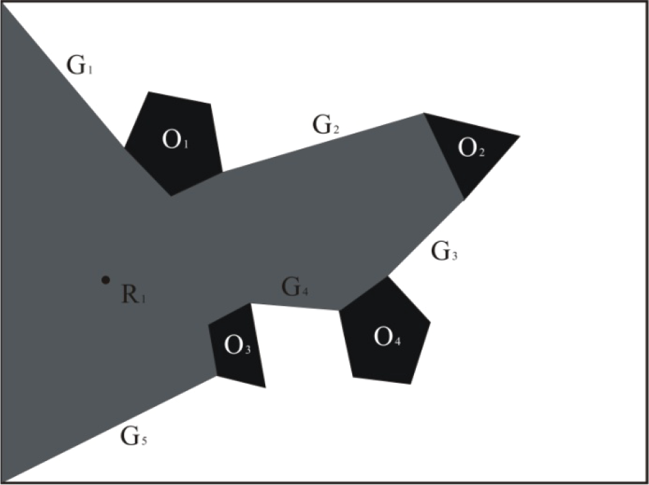
The visible region forms a visibility-based polygon

Fig. 2

Graph representation

Fig. 3

Cells after decomposition

The formal algorithm 1 presents a coverage algorithm for single robot, GU is a FILO stack of unvisited gates, GV is a list of visited gates, GRAPH is a data structure of our graph representation, records cells and gates and connection relationships between cells. In next section we will further discuss how these tasks are fulfilled by a team of robots.

Algorithm 1:

Let GU={Ø}, GV={Ø}, GRAPH={Ø};

Observe and form a cell, push all new gates into GU

Add the cell to GRAPH, then inspect current cell;

If GU={Ø}, go to 11, else continue next steps;

Pop a gate from GU, then add it to GV;

Go to the middle of the gate, then observe and form a new visible cell, make a set operation NC=Connect(NC-INTER) if it intersect with other cells in GRAPH (NC is the new cell, INTER is its intersection part, Connect returns parts connected with current gate);

If NC={Ø}, go to 10, else continue next steps;

Add the modified NC and the gate which connects NC and previous cell to GRAPH; find all gates in front of robot, check gates, if there are any gates already in GU, add these gates to GRAPH and move them to GV, other new gates which are not in GU will be added to GU;

Inspect current new cell NC;

Go to 4;

end.

In step 2 and 6, formed cell is a polygon whose vertices are organized as anticlockwise order, so it is important to order vertices from different obstacles. A simple rule is derived from the property of visibility-based polygon as algorithm 2 shows, P stores vertices ordered, n is total number of cell vertices, VE_n denotes a line of sight vector from the center of a robot to nth vertex, A_m (m@[1,n]) is the angle of corresponding vector VE_m.

Algorithm 2:

Set P={V₁, V₂, …, V_n};

Construct n vectors VE₁, VE₂, …, VE_n, and corresponding angle A₁, A₂, …, A_n;

Sort A₁, A₂, …, A_n in ascended order, at the same time the corresponding position of V_m (m@[1,n]) in P is also changed to the equal position of An in new order; if two angle is equal, keep their adjacency with vertices of same obstacle.

end.

It is reasonable that vertices of the cell polygon are sorted as ascended order by angles of line of sight, because a visibility-based polygon which is represented as a series of anticlockwise visible vertices, its angles of line of sight have natural ascended order, it can be obviously viewed from Fig. 4. Construction of a polygon cell couldn't be so easy unless the property of natural order. It is also reasonable in step 6 of algorithm 1 that robot directly goes to the middle of gate for the visibility of that gate. How to form a cell is slightly different between step 2 and step 6, the cell of step 6 only include vertices whose line of sight are in front of robot, because vertices behind the gate have been formed into old cell.

Fig. 4

Natural ordered vertices of a visibility-based polygon

In an unknown environment, the construction of graph representation is incrementally built with the discovery of new cells. In algorithm 1, the exploration is indeed a depth first search maintained by GU and GV, when new cells and gates are discovered, new vertices and edges are added to GRAPH, GRAPH organizes the relationships of cells and is utilized to describe the partially observed world. The completeness of Algorithm 1 is guaranteed by depth first search and it will end within limited time for finiteness of gates number. The collision free path comprises all line segments from observation points (start position and middle points of all gates) to its visible gates, robot searches feasible path in it for motion of coverage planning, many general or heuristic search algorithms can do it.

4. Multi-robot coverage

When multiple robots are introduced, things are more complex, especially they are distributed, there are needs of gates allocation and environmental data synchronization. Algorithm 3 derives a solution for the distributed multi-robot systems from algorithm 1. Robots are put together in a location of workspace at the beginning of coverage. ID is a integer identity of a robot, the less the ID, the greater the priority of robot.

Algorithm 3:

Let GU={Ø}, GV={Ø}, GRAPH={Ø};

Confirm current team members in communication range;

Compare priority with team members, if priority is the highest of current team, observe and form a cell, push all new gates into GU, add the cell to GRAPH, then pass GU and GRAPH to others, else receive them from the highest priority robot (R_j (j@[1,k]));

If GU={Ø}, go to 12, else continue next steps;

If my ID is j, inspect current cell boundary if no another robot does it, choose a gate from GU for next step; else pop a gate in GU which is not chosen by higher priority robot, if no gates left, follow the robot whose priority is minimum in robots owned gates and choose the same gate with the robot;

Pop all chosen gates in last step, add them to GV; respectively go to the middle of gate chosen by self;

Compare priority with team members at same gate; if priority is the highest of current team, observe and form a cell (like step 6–7 in algorithm 1), then continue next steps; else jump to step 10;

When other teams are observed in the new cell, re-select the highest priority robot R_j from all current visible teams and merge them, if j is unchanged, continue next steps, else jump to step 10;

R_j gather information of inspected cells by teams, update GU and GV, gates in GU which accessed by other robots are moved into GV, then add new cells and gates into GRAPH and update modified cells, if necessary reorganize it;

Update information through the highest priority robot R_j, if ID is not j;

Go to 4;

end.

The feasible paths of multi-robot are same with single robot, so when two teams travel on same line segment, collisions maybe occur. We use reactive method to avoid collisions, when two teams travel toward each other they are follow the rule of keeping to the right of road. Communication and share&mergence of information are heavy burden for highest priority robot, so they only happen when there are teams at observation points at the cost of repeated coverage of some teams.

5. Experimentation and evaluation

We use the map which has 20mx15m rectangle environmental boundary as Fig. 1 showed to evaluate algorithm 3 in a simulated implementation, robots number is from 1 to 5, the average results are presented at Table 1. Total length is the path length travelled by all robots, Repeated coverage length is the path length which is repeated travelled by robots, rate of repeated coverage (RRC) is calculated by the division of them.

Table 1.

Statistic results of coverage

Number of robots	Total length (m)	Rate of repeated coverage
1	327.8	10.1%
2	311.5	5.4%
3	306.5	3.9%
4	309.8	4.9%
5	320.7	8.1%

As the simplicity of map, above results may not represent any circumstance, yet the relationship between RRC and number of robots could be exposed. RRC is decreasing with increase of robot number because interaction between teams eliminates some backtracking, while RRC is increasing after turning point where robot number is 3 for the reason of following behavior of some robots. Furthermore it can be observed that turning point could be determined by average gate number of a cell and number of robots, when number of robots is less than average gate number, RRC is decreasing with increase of robot number, otherwise RRC is increasing.

6. Conclusion

The paper presents an algorithm for multi-robot boundary coverage based on a single robot boundary coverage algorithm. The visibility-based decomposition powers robots to incrementally construct unknown environment and describe it easily. The representation of environment is a graph data structure which gives a description of partially observed world and feasible collision free paths, its depth first search makes a guarantee of coverage completeness. Communication provides a tool for environmental information synchrony, information share and synchrony are conducted by a highest priority robot which is dynamically selected. Strategies of boundary coverage are our main concern, therefore the low level path finding and collision avoiding between robots are only introduced briefly.

There are still lots of works remained to improve the multi-robot boundary coverage algorithm. For example, if robot team can communicate when they meet at midway of going to gates, some repeated coverage path could be reduced. The computational cost of brute-force environmental information mergence need to be improved. How to choose optimal number of robots is also a problem in an unknown environment. Moreover when robots enter the real world, uncertainty of environmental information brings huge difficulties to environmental information mergence. These issues are subjects of our future researches.

References

Agmon

Hazon

; and Kaminka

G. A.

(2006). Constructing Spanning Trees for Efficient Multi-Robot Coverage, Proceedings of IEEE International Conference on Robotics and Automation, pp. 1698–1703, May 15–19, 2006.

Butler

Z. J.

Rizzi

A. A.

Hollis

R. L.

(2000). Cooperative coverage of rectilinear environments, Proceedings of IEEE International Conference on Robotics and Automation, Vol. 3, pp. 2722–2727, 24–28 April, 2000.

Choset

(a) (2000). Coverage of Known Spaces: The Boustrophedon Cellular Decomposition, Autonomous Robots, Volume 9, Number 3, 2000, pp. 247–253, ISSN:.

Choset

(b) (2001). Coverage for robotics-a survey of recent results. Annals of Mathematics and Artificial Intelligence, Vol. 31, October, 2001, pp. 113–126, ISSN: 1012-2443.

Cortes

Martinez

Karatas

Bullo

(2004). Coverage control for mobile sensing networks. IEEE Transactions on Robotics and Automation, Volume 20, Issue 2, April 2004, pp. 243–255, ISSN: 1042-296X.

Easton

and Burdick

(2005). A Coverage Algorithm for Multi-robot Boundary Inspection, Proceedings of the 2005 IEEE International Conference on Robotics and Automation, pp. 727–734, 18–22 April 2005, Barcelona, Spain.

Gabriely

and Rimon

(2001). Spanning-tree based coverage of continuous areas by a mobile robot, Proceedings of IEEE International Conference on Robotics & Automation, pp. 1927–1933, 2001.

Hazon

and Kaminka

G. A.

(2005). Redundancy, Efficiency, and Robustness in Multi-Robot Coverage. Proceedings of IEEE International Conference on Robotics and Automation, pp. 735–741, 18–22 April, 2005.

Keil

J. M.

and Sack

J. R.

(1985). Minimum Decomposition of Polygonal Objects, Computational Geometry, pp. 197–216, Elsevier Science Publishers B.V., North Holland.

10.

Latimer

Srinivasa

Lee-Shue

Sonne

Choset

& Hurst

, Towards Sensor Based Coverage with Robot Teams, Proceedings of IEEE International Conference on Robotics & Automation, pp.961–967, Washington, DC, May 2002.

11.

Rekleitis

Lee-Shue

Peng

A. N.

& Choset

(2004). Limited communication, multi-robot team based coverage. Proceedings of IEEE International Conference on Robotics and Automation, Volume 4, pp. 3462–3468, Apr 26-May 1, 2004.

12.

Thrun

(2002). Robotic Mapping: A Survey, Carnegie Mellon University technical report, CMU-CS-02-111, Available from: http://reports-archive.adm.cs.cmu.edu/cs2002.html, Accessed: 2006-12-08.

13.

Wager

I. A.

Lindenbaum

& Bruckstein

A. M.

(a) (1999). Distributed covering by ant-robots using evaporating traces. IEEE Transactions on Robotics & Automation, Vol. 15, No. 5, 1999, pp. 918–933, ISSN: 1042-296X.

14.

Wager

I. A.

Lindenbaum

& Bruckstein

A. M.

(b) (2000). MAC vs. PC – determinism and randomness as complementary approaches to robotic exploration of continuous unknown domains. The International Journal of Robotics Research, Vol. 19, No. 1, 2000, pp. 12–31, ISSN: 0278-3649.

15.

Williams

and Burdick

(2006). Multi-robot boundary coverage with plan revision, Proceedings of 2006 IEEE International Conference on Robotics and Automation, pp. 1716–1723, May 15–19, 2006, Orlando, Florida.

16.

Yamauchi

(a) (1997). A frontier-based approach for autonomous exploration, Proceedings of IEEE International Symposium on Computational Intelligence in Robotics and Automation, pp. 146–151, 10–11 July, 1997.

17.

Yamauchi

Schultz

Adams

(b) (1998). Mobile robot exploration and map-building with continuous localization, Proceedings of IEEE International Conference on Robotics and Automation, Volume 4, pp. 3715–3720, 16–20 May, 1998.

18.

Yamauchi

(c) (1998). Frontier-based exploration using multiple robots. In Proceedings of the Second International Conference on Autonomous Agents, pp. 47–53, 1998.

19.

Zheng

Jain

Koenig

& Kempe

(2005). Multi-robot forest coverage, Proceedings of IEEE International Conference on Intelligent Robots and Systems, pp. 3852–3857, 2–6 Aug, 2005.

A Visibility-Based Algorithm for Multi-Robot Boundary Coverage

Abstract

Keywords

1. Introduction

2. Preliminary description

3. Visibility-based decomposition and coverage

4. Multi-robot coverage

5. Experimentation and evaluation

6. Conclusion

References