Sage Journals: Discover world-class research

Abstract

This article introduces multi-robot strategies making multiple robots explore an unknown environment in a cooperative manner. Our exploration strategies do not require global localization of a robot or a node. Multiple robots build a Voronoi diagram as a topological map of the environment, while deploying sensor nodes which can sense and communicate. As the sensor network built by one robot meets the network built by another robot, both robots can exchange data with each other. The robots then use the merged sensor network to protect the environment. We introduce an intruder capture algorithm assuming that a robot is able to access any intruder’s location utilizing the sensor network. This algorithm is robust to time delay in information sharing utilizing the sensor network. Utilizing the algorithm, we derive upper bounds on the number of robots needed to capture every intruder in the environment. This article proves that the minimum number of robots needed can be computed by finding proper edge covers of the dual graph of the Voronoi diagram.

Keywords

Multi-robot exploration and mapping Voronoi diagram graph theory sensor network intruder capture graph clear visible intruder

Introduction

Operating multiple robots in a complex and dangerous environment needs the support from a sensor network that can detect environmental changes and also relay data among the robots. Sensor network becomes feasible due to the development of small sensor nodes, such as the Berkeley Motes.¹ Research advances in sensor networking^2,3 showed that small sensor nodes can be positioned to construct a sensor network for supporting rescue workers.

However, building a sensor network in dangerous environments is not easy. As an autonomous method for building a sensor network, mobile sensor nodes can be used.⁴ But, considering the time spent and power loss due to the maneuver of each node, it is desirable to minimize the maneuver of a sensor node.

As a method to construct a sensor network efficiently, this article presents the multi-robot networking and exploration strategy called the Simultaneous Cooperative Networking and exploration (SCN) strategies.⁵ In SCN strategies, each robot uses the boundary expansion (BE) algorithms in our previous work⁶ to construct a Voronoi diagram of the environment while deploying sensor nodes (Voronoi diagrams were widely used as a topological map.^7

–11 Also, a Voronoi diagram was used in coverage problems of sensor networks.¹²). The robots start exploration at arbitrary locations, thus they may not be able to exchange data with each other initially. Deployed sensor nodes form a network allowing the robots to exchange data with other robots. Moreover, sensor deployment enables time-efficient networking while exploration. Our exploration strategies do not need global localization of a robot or a node (Localization of a robot or a sensor node is a critical problem to solve in both robotics and sensor networks.^{13

–21}). As a result of SCN strategies, a sensor network and a topological map are created simultaneously.

The resulting sensor network and the topological map, represented by Voronoi diagrams, are utilized by the robots to coordinate their motions to secure the environment. Because of obstacles, both intruders and robots are restricted to traverse a passage between two obstacles. This article considers the case in which the weapons on robots are powerful sufficient to cover the width of a passage between obstacles. This case, we can consider a simplified scenario where searchers and intruders traverse Voronoi edges. We present an intruder capturing game in the Voronoi diagram, assuming that a robot is able to access any intruder’s location utilizing the sensor network.

Previous research on pursuit-evasion games on graphs, as presented in the study by Parsons²² and Kolling and Carpin,²³ mentioned that successful capturing strategies require guarding a passage to block escape of an intruder. In this article, we obtain bounds on the number of guards needed to capture every intruder on a Voronoi diagram assisted by the sensor network. The problem tackled in this article is similar to that in the study by Seymour and Thomas²⁴ and Richerby and Thilikos,²⁵ since an intruder is visible to a robot. Here, a robot uses the sensor network to detect an intruder.

While general graphs were considered in the works of Seymour and Thomas²⁴ and Richerby and Thilikos,²⁵ we focus on capturing intruders in a Voronoi diagram. We introduce an intruder capture algorithm assuming that a robot is able to access any intruder’s location utilizing the sensor network. This algorithm is robust to time delay in information sharing utilizing the sensor network. Based on the algorithm, we prove that the minimum number of searchers needed can be computed by finding proper edge covers of the dual graph of the Voronoi diagram. As far as we know, our article is novel in deriving the relationship between the number of robots needed and a Voronoi diagram.

The article is organized as follows: Second section reviews works related to our article. Third section reviews preliminaries and background information. Fourth section presents how to build the sensor network in a cooperative manner. Fifth section provides the intruder capture algorithm based on sensor networks. Next, sixth section presents MATLAB simulation results. Finally, seventh section presents conclusions.

Related works

Our article is closely related to multi-robot networking strategies introduced in the literature.^5,26
–28 Multi-robot networking algorithms in the literature^5,26
–28 require that a robot stores the adjacency matrix associated to all vertices and searches for a closest unexplored vertex utilizing the matrix. Searching for a closest unexplored vertex can be computationally burdensome especially in the case where there are many vertices.

In SCN algorithms, each robot only stores the circularly linked list structure, called the enclosing boundary (EB; “BE algorithm” section presents the rigorous definition of the EB), representing the boundary of the explored area thus far. Since a robot does not have to store the adjacency matrix associated to all vertices, our algorithms require less memory compared to other multi-robot networking algorithms in the literature.^5,26,27 Also, a robot does not have to search for a closest unexplored vertex.^5,26,27 As far as we know, our article is novel in not searching for a closest unexplored vertex, in the literature on multi-robot exploration.

Complexity analysis section analyzes the computational complexity of both our algorithms and other algorithms searching for a closest unexplored vertex. We show that as the network size increases, the complexity of our algorithms decreases compared to other algorithms searching for a closest unexplored vertex.

The EB was also used in our previous papers.^5,6 Kim et al.⁶ considered one robot exploration, while Kim et al.⁵ considered multi-robot exploration and networking. Note that both SCN algorithm in this article and the algorithm in Kim et al.⁶ do not require that a robot stores the adjacency matrix associated to all vertices. Our article extends Kim et al.’s⁶ work to multi-robot exploration and networking by letting multiple robots construct the sensor network in a cooperative manner. The multi-robot networking strategy in Kim et al.⁵ requires that a robot stores the adjacency matrix associated to all vertices. Kim et al.⁵ require this full adjacency matrix, since a robot has to search for a closest unexplored vertex in the case where a blocking of EB occurs. Utilizing SCN algorithm in this article, this blocking does not happen, since we merge two EBs if they intersect while satisfying certain conditions. Under SCN algorithm, a robot does not have to search for a closest unexplored vertex, as in the study by Kim et al.⁵

Suppose that the sensor network is completely built utilizing multiple robots. We further present an intruder capture algorithm in the Voronoi diagram of the environment, assuming that a robot is able to access any intruder’s location utilizing the sensor network.

The graph searching problem was originated from Parsons’ study.²² There are many papers on graph search problems.^{22,24
–26,29

–40} Several authors tackled clearing a weighted graph.^{23,30,33,41,42} In a weighted graph, the weight of an edge or a vertex is a cost describing the clearing requirement of the edge or the vertex. Among many papers, our article is closely related to the helicopter cops game in the study by Seymour and Thomas²⁴ and Richerby and Thilikos.²⁵ In this game,^24,25 a cop is able to access robbers’ locations as if the cop utilizes a helicopter. Thus, an intruder is visible by a cop. Furthermore, a cop can jump from one vertex to another. We say that a cop captures a robber if the cop visits the node on which the robber exists.

The problem formulated in this article is similar to that in the study by Seymour and Thomas²⁴ and Richerby and Thilikos,²⁵ since this article assumes that an intruder is visible to a searcher utilizing the sensor network. In this article, a robot traverses graph edges continuously, which is distinct from the study by Seymour and Thomas²⁴ and Richerby and Thilikos.²⁵

While general graphs were considered in the works of Seymour and Thomas²⁴ and Richerby and Thilikos,²⁵ this article is focused on capturing intruders on a Voronoi diagram. A Voronoi diagram has been widely used to represent a plane structure such as a floor in buildings.⁴¹ A Voronoi diagram has also been used as a topological map representing a workspace with many obstacles.^6,8,41 We introduce an intruder capture algorithm assuming that a robot is able to access any intruder’s location utilizing the sensor network. This algorithm is robust to time delay in information sharing utilizing the sensor network. Utilizing the algorithm, we prove that the minimum number of robots needed can be computed by finding proper edge covers of the dual graph of the Voronoi diagram. As far as we know, our article is novel in deriving the relationship between the number of robots needed and a Voronoi diagram.

Preliminaries and background

In this section, we discuss background information which are used to present our contributions.

Graphs

We review graph theory⁴³ used in this article. A graph G is a set $G = (N (G), E (G))$ . Here, $N (G)$ is the set of vertices in G, and $E (G)$ is the set of edges in G. A subgraph is a subset of G. A path is an alternating sequence of vertices and edges in a graph such that each vertex is adjacent to the edge immediately before and after it in the sequence. We say that G is connected in the case where there exists a path between any two vertices in G. A cycle denotes a path with identical starting and ending vertices. A tree graph T is a connected graph containing no cycles. A branch of T at n is the maximal subgraph of T, such that n has degree one in the subgraph.

A plane graph is a graph embedded in the plane without crossing edges. A face of a plane graph is the maximal region of the plane that is surrounded by a cycle of edges but contains no vertex which belongs to any edge of the embedded graph. For example, a two-dimesional Voronoi diagram is a plane graph in which each Voronoi cell is a face. G* is called the dual graph of a plane graph G in the case where G* is constructed as follows: each face of G is represented by a node in G*, and each edge shared by two adjacent faces of G is represented by an edge in G*. G* is also a plane graph. For any plane graph G, its boundary ∂G is a set of edges and nodes that separate the region enclosed by the graph with the rest of the plane. A cycle in a plane graph separates the plane into two regions, the region inside the cycle and the region outside the cycle. If a plane graph contains a cycle, then its boundary must also contain a cycle. If G contains no cycles, then all edges and nodes are on the boundary, for example, ∂G = G.

A matching M in G is defined as a set of pairwise non-adjacent edges. In other words, no two edges are adjacent to a common vertex. A maximum matching is a matching having the largest possible number of edges. A maximum matching can be calculated in polynomial time utilizing the Edmonds’ Blossom algorithm.^44,45

An edge cover of a plane graph G, represented by $C (G)$ , is a subset of edges such that every vertex in G is adjacent to an edge in $C (G)$ . A minimum edge cover is the one that contains the fewest number of edges among all edge covers. A minimum edge cover can be found in polynomial time by finding a maximum matching followed by extending the matching greedily until all vertices are covered.

A perfect matching in G is a minimum edge cover in which no vertex is shared by any pair of edges. If a perfect matching exists, then its cardinality is $\frac{| N (G) |}{2}$ , where $| N (G) |$ is the number of vertices in the graph G.

The environment and its Voronoi diagram

Consider an environment $W \subset R^{2}$ . ∂W, the boundary of the environment, is a simple and closed curve without self-intersection. Let O₁,O₂,… $O_{M - 1}$ be M − 1 obstacles in W. O_M is a “virtual” obstacle bounding the environment, that is, $\partial W \subset \partial O_{M}$ .

Obeying the conventions in the literature on Voronoi diagrams,^{8,10,46

–49} a Voronoi cell V_i for an obstacle O_i is the set of points which are closer to O_i than to O_j where j ≠ i. ∂V_i is the boundary of the Voronoi cell V_i. This definition on Voronoi cells was also used in the study by Kim et al.^5,6

The following assumptions, which were also used in the study by Kim et al.,^5,6 are used.

Assumption 1

∂V_i of every Voronoi cell V_i is closed and simple.

Assumption 2

$\cup_{i = 1}^{M} (V_{i} \cup \partial V_{i}) = W .$

The Voronoi diagram G is a plane graph and denotes the union of all cell boundaries. A Voronoi edge E_ij is an edge shared by two Voronoi cells V_i and V_j. A Voronoi vertex is a node where more than two Voronoi edges meet.

BE algorithms

Kim et al.⁶ introduced the BE algorithms to build the Voronoi diagram of the environment utilizing one robot.

We reviewed BE algorithms in Kim et al.⁶ briefly. We need to introduce several definitions in the study by Kim et al.⁶ An intersection P is a point satisfying the following conditions:

There exists a circle, whose center is P, intersecting obstacle boundary at more than two points. These points are denoted as the closest points at the intersection. In the case where the robot is located at an intersection, the closest points are the points which have local minimal distances to the robot.

The interior of the circle does not contain a point of an obstacle, that is, the circle is tangential to an obstacle.

An intersection circle is a circle satisfying the above conditions (see Figure 1). The line segments connecting the intersection and the closest points divide the intersection circle into sectors. Each sector is the “pie-shaped area” inside the intersection circle (see Figure 1).

Figure 1.

The robot is at P. The closest points divide the intersection circle into sectors. Sector i is adjacent to the sector i − 1 in the counter-clockwise direction.

Consider the case in which the robot traverses E_ij until it meets P, as depicted in Figure 1. Then, the robot encounters two closest points on ∂O_i and ∂O_j, respectively, since $P \in E_{i j}$ . The sector having these two closest points as its end points is called the sector 0 at P. The robot moves through sector 0 to reach P. Sector 0 is a starting sector for indexing the other sectors. Consider the case in which there are n sectors in the intersection circle. We index the sectors in the counter-clockwise direction starting from sector 0. q satisfies $0 \leq q \leq n - 1$ . See Figure 1 for an illustration.

In the case where two end points of a sector exist on the identical obstacle boundary, then the sector is a blocked sector (see Figure 1). An open sector (sectors 1 and 3 in Figure 1) is a sector that is neither sector 0 nor a blocked sector. If an intersection has an open sector which has not been visited by the robot, then the intersection is set as unexplored. Otherwise, the intersection is set as explored.

In BE algorithms, the robot circles around an obstacle, say O_j, to its right while traversing ∂V_j. To enable this circling, the robot applies the sector selection rule as follows:

In the case where the robot meets an intersection that is not on the EB, then the robot searches for an open sector in the counter-clockwise direction starting from sector 0. In the case where an open sector is found, the robot moves through the found open sector.

For example, consider the case in which the robot reaches P as depicted in Figure 1. Then, under the sector selection rule, the robot chooses sector 1 to circle around O_j to its right.

Consider the case in which the robot traverses Voronoi edges utilizing the tracking controller in Kim et al.⁶ Utilizing the above sector selection rule, the robot can circle around an obstacle, say O_j, to its right while traversing ∂V_j. We denote this cycle as the initial enclosing boundary B₀.

B_k denotes EB that is updated with k + 1 steps. Since one obstacle is added at each step, B_k encloses k + 1 obstacles.

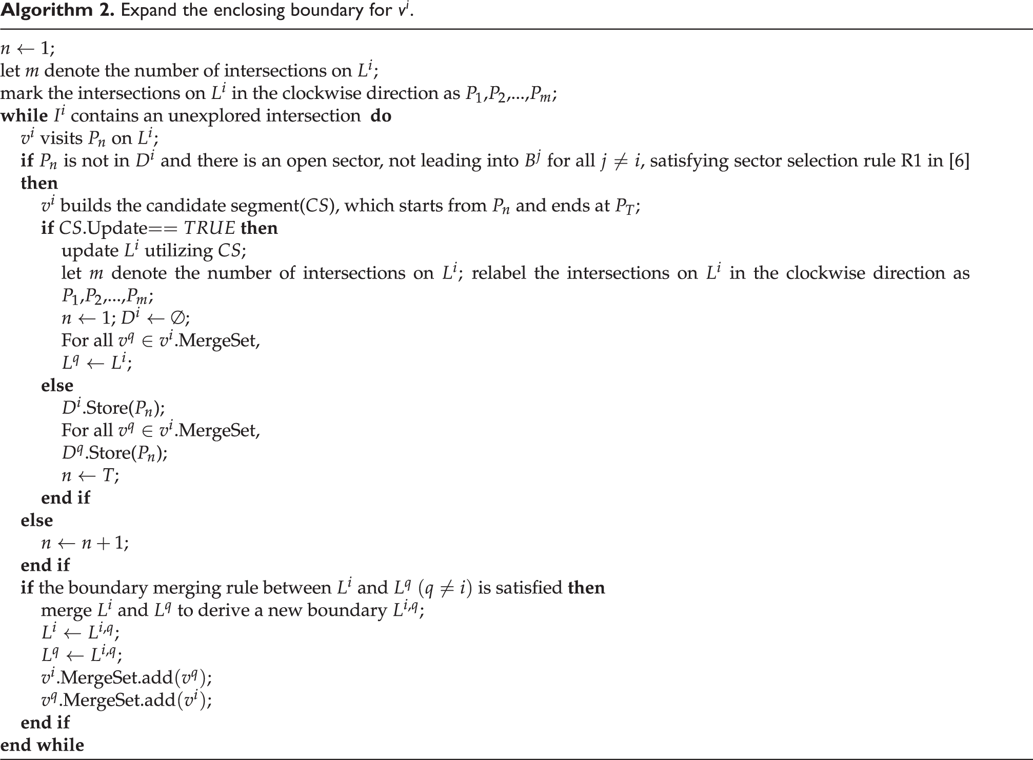
To update the EB, the robot traverses EB until it visits an unexplored vertex, say head. Then, the robot at the head traverses an unexplored edge out of EB, followed by circling around an obstacle to its right. Here, the sector selection rule is used to circle around an obstacle to its right. Since each Voronoi cell boundary is a cycle, the robot meets EB again. Let tail denote the point where the robot intersects EB again. Let candidate segment (CS) denote the robot’s path out of EB such that two end nodes of the path are on EB. See Figure 2 for an illustration.

Figure 2.

The case in which the EB expands. EB: enclosing boundary.

We next present the boundary updating rule, which decides when we update EB utilizing the CS. The rule is given as follows:

Consider the case in which no unexplored intersection exists strictly between head and tail along the segment of EB in the clockwise direction. In this case, the segment of EB from head to tail is replaced by CS.

Consider the case in which the current EB is B_k. Figure 2 depicts the case in which no unexplored intersection exists strictly between head and tail along the segment of EB in the clockwise direction. This implies that the boundary updating rule is met. In this case, we update B_k to $B_{k + 1}$ by replacing the segment of EB from head to tail by CS.

During the process of updating EB, all unexplored vertices only exist on or outside EB. The algorithms end as EB encircles all obstacles except for O_M. Thus, BE algorithms end in finite time resulting in a complete Voronoi diagram. Because of page limits, we do not present entire BE algorithms in this article. See Kim et al.⁶ for a detailed explanation of BE algorithms.

Exploring while networking

BE algorithms can be performed by multiple robots at the same time to cooperatively explore an environment. N_v denotes the number of robots. Let us denote each robot as $v^{j} (j \leq N_{v})$ . v^j traverses Voronoi edges by running BE algorithms and stores the EB B^j.

Every robot v^j carries sensor nodes that can detect a neighborhood around each node, while communicating with a robot or a node nearby. Here, note that a node deployed by a robot v^j can communicate with a nearby node deployed by v^q, where q ≠ j. Sensor nodes are positioned at Voronoi vertices or on long Voronoi edges to relay data between things (including both robots and nodes). These sensor nodes then form a sensor network that serves two purposes: (1) to relay data between things (including both robots and nodes) and (2) to provide a movement direction for a robot visiting the node.

Based on the results in the study by Souryal et al.² and Liu et al.,³ we assume that the sensor network operates once the nodes are deployed. We also assume that each sensor node has its unique ID. Thus, a robot visiting a node can localize itself based on the node’s ID.

Each sensor node stores data regarding whether the node has been explored or not. Each node at an intersection on EB stores the Voronoi edge direction along EB. By checking the Voronoi edge direction along EB, a robot can expand its EB, as presented in Algorithms 1 and 2.

Note that global localization of a node or a robot is not required in our algorithms.

Boundary merge

Two sensor nodes laid out by distinct robots are connected once the nodes are close to each other. When a robot v^j encounters a sensor node which can communicate with a node laid out by another robot v^q, v^j can use the sensor network built by v^q. Thus, v^j can communicate with v^q utilizing the network. Note that v^j does not have to meet v^q to exchange data with each other.

Each robot v^j maintains B^j and expands B^j such that the area inside B^j does not overlap with that inside B^q, where q ≠ j. It may happen that B^j intersects with B^q, where q ≠ j. Consider the case in which B^j intersects B^q along Voronoi edges, say $ES = B^{j} \cap B^{q}$ . In the case where ES is connected and no unexplored intersection exists strictly inside ES, then we merge B^j and B^q to get $B^{j, q} = (B^{j} \ ES) \cup (B^{q} \ ES)$ , the enclosing boundary for both v^j and v^q. B^j,q is depicted in Figure 3. There is no unexplored Voronoi vertex in B^j as well as in B^q. Hence, there is no unexplored Voronoi vertex inside B^j,q.

Figure 3.

$ES = B^{j} \cap B^{q}$ is connected, and no unexplored intersection exists strictly inside ES. $B^{j, q} = (B^{j} \ ES) \cup (B^{q} \ ES)$ .

We also merge two enclosing boundaries in the following situation: B₀ constructed by one robot is identical to B₀ constructed by another robot. This situation may happen in the case where an obstacle to the right of one robot v^j is identical to an obstacle to the right of another robot v^q. In this case, B^j and B^q are merged to get $B^{j, q} = B^{j} = B^{q}$ .

In summary, we introduce the boundary merging rule as follows:

Consider the case in which $ES = B^{j} \cap B^{q}$ is connected and no unexplored intersection exists strictly inside ES. In this case, merge B^j and B^q to get $B^{j, q} = (B^{j} \ ES) \cup (B^{q} \ ES)$ .

In the case where $B^{j} = = B^{q}$ , then $B^{j, q} = B^{j} = B^{q}$ .

$B^{j, q}$ is the enclosing boundary for both v^j and v^q. Once $B^{j, q}$ is built, we say that v^j and v^q are merged. Once v^j and v^q are merged, we add v^q to the set of robots that are merged to v^j. Also, we add v^j to the set of robots that are merged to v^q.

Once v^j and v^q are merged, both v^j and v^q traverse $B^{j, q}$ while expanding $B^{j, q}$ utilizing BE algorithms.⁶ SCN algorithms terminate when all Voronoi vertices have been explored.

SCN algorithms are presented in Algorithms 1 and 2. Table 1 shows the data structures and operations used in these algorithms. Intersection, sector, sector selection rule, and disabled intersection set in these algorithms are presented in Kim et al.⁶ Algorithms 2 and 3 do not present how to build the CS in detail. See Algorithm 2 in Kim et al.⁶ for a detailed explanation of how to build the CS.

Algorithm 1.

Construct the initial enclosing boundary for vⁱ.

Algorithm 2.

Expand the enclosing boundary for vⁱ.

Table 1.

Data Structure.

Lⁱ: the circular linked list presenting Bⁱ.

CS: the singly linked list presenting the candidate segment.

CS.Update: if the boundary updating rule is satisfied, then return TRUE. Otherwise, return FALSE.

Dⁱ: the disabled intersection set of Bⁱ.

Set.Store(Data): store Data in Set.

vⁱ.MergeSet: set of robots that are merged to vⁱ.

vⁱ.MergeSet.add(v^q): add v^q to vⁱ.MergeSet.

Algorithm 3.

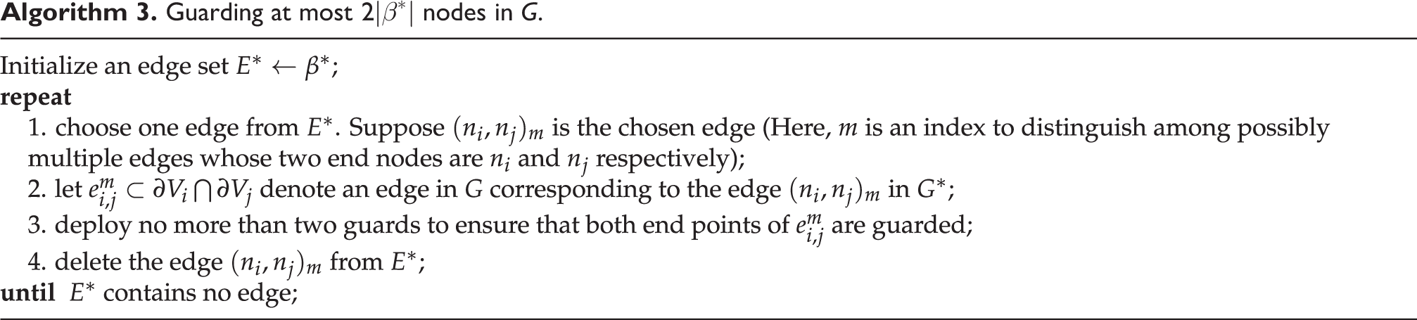
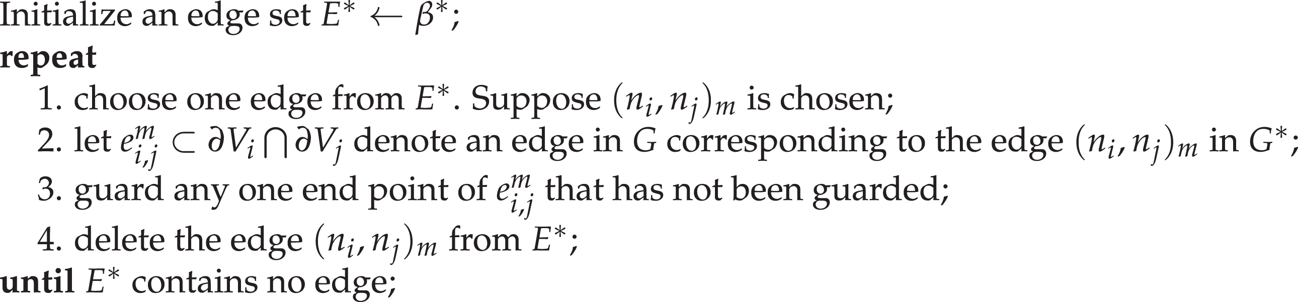
Guarding at most $2 | β^{*} |$ nodes in G.

Complexity analysis

We analyze the complexity of SCN algorithms in the case where a robot vⁱ is connected to N nodes utilizing multi-hop communication.

Other multi-robot networking algorithms in the literature^5,26,27 require that vⁱ stores the adjacency matrix associated to all vertices and searches for a closest unexplored vertex utilizing the matrix. Searching for a closest unexplored vertex can be costly especially in the case where there are many vertices. Dijkstra’s algorithm is commonly used for this search. Since vⁱ is connected to N vertices, the complexity of this Dijkstra’s algorithm is $O (N^{2})$ .

In SCN algorithms, a robot vⁱ does not store the adjacency matrix associated to all vertices. vⁱ only stores the data on vertices along Bⁱ and updates Bⁱ if necessary. Thus, our algorithms require less memory compared to other multi-robot networking algorithms in the literature.^5,26,27

SCN algorithms use two rules for exploration and networking: boundary updating rule and boundary merging rule. These two rules search for an unexplored vertex along EB, thus can be implemented utilizing the data of vertices on EB, whose structure is a circularly linked list. vⁱ does not require the data of vertices strictly inside EB.

Since vⁱ is connected to N vertices, there are at most N vertices inside EB. Considering a rectangular boundary, the number of vertices along EB can be approximated as $O (\sqrt{N})$ . Since vⁱ searches for an unexplored vertex along EB, the complexity of this search is also $O (\sqrt{N})$ . See that the complexity of our algorithms is much lower than $O (N^{2})$ , that is, the complexity of Dijkstra’s algorithm. This implies that as the network size N increases, the complexity of our algorithms decreases compared to other multi-robot networking algorithms in the literature.^5,26,27

Performance analysis

We estimate the exploration time utilizing our algorithms. Consider unit speed robots exploring W. T denotes the maximum time required for a robot to circle around one Voronoi cell.

Lemma 1 considers the case in which we use a single robot for exploration. The proof of Lemma 1 is similar to that of Theorem 3 in the study by Kim et al.⁶ Thus, we omit the proof here.

Lemma 1

Consider a robot that has constructed an enclosing boundary enclosing M obstacles. The time spent is bounded by $T (\frac{1}{2} {(M - 1)}^{2} + \frac{3}{2} (M - 1) + 1)$ .

Next, we consider the case in which two robots vⁱ and v^j are deployed. We prove the following theorem.

Theorem 1

Consider the case in which two robots vⁱ and v^j are deployed in W with M obstacles. Suppose that Bⁱ expands with k₁ steps and that B^j expands with k₂ steps before they are merged. Let $k^{*} = max (k_{1}, k_{2})$ . $k_{n} = k_{1} + k_{2} + 2$ . Also, let $T^{*} = T (\frac{1}{2} {(k^{*})}^{2} + \frac{3}{2} (k^{*}) + 1)$ . The time spent to explore W is bounded by $T^{*} + 2 T (M - k_{n} - 1) + T / 2 (k_{n} + M - 2) (M - 1 - k_{n})$ .

Proof

Suppose that Bⁱ expands with k₁ steps and that B^j expands with k₂ steps before they are merged. Once Bⁱ expands with k₁ steps, it encloses $k_{1} + 1$ obstacles. The time spent is bounded by $T_{1} = T (\frac{1}{2} {(k_{1})}^{2} + \frac{3}{2} (k_{1}) + 1)$ utilizing Lemma 1. Once B^j expands with k₂ steps, it encloses $k_{2} + 1$ obstacles. The time spent is bounded by $T_{2} = T (\frac{1}{2} {(k_{2})}^{2} + \frac{3}{2} (k_{2}) + 1)$ utilizing Lemma 1.

Since $B^{i, j}$ encloses $k_{n} = k_{1} + k_{2} + 2$ obstacles, let $B_{k_{n}}$ denote $B^{i, j}$ for convenience. $B_{k_{n}}$ can be constructed within the time interval $T^{*} = T (\frac{1}{2} {(k^{*})}^{2} + \frac{3}{2} (k^{*}) + 1)$ in which $k^{*} = max (k_{1}, k_{2})$ .

Next, we derive the time spent to generate $B_{k_{n} + 1}$ from $B_{k_{n}}$ . Suppose that $B_{k_{n}}$ is built and that the robot is at the tail of CS for constructing $B_{k_{n}}$ .

Utilizing Theorem 2 in Kim et al.,⁶ at least one Voronoi cell, which exists outside $B_{k_{n}}$ and meets the perimeter of $B_{k_{n}}$ , is an addable obstacle Q. Q is an obstacle that will be inside $B_{k_{n} + 1}$ . The robot traverses $B_{k_{n}}$ until meeting the starting point (head) of $\partial V (Q) \cap B_{k_{n}}$ . The robot’s maximal traversal distance until meeting the head of $\partial V (Q) \cap B_{k_{n}}$ is bounded by the length of $B_{k_{n}}$ . The number of Voronoi cells, which are enclosed by $B_{k_{n}}$ , is $k_{n} + 1$ , and the robot moves with unit speed. Hence, the length of $B_{k_{n}}$ is bounded by $(k_{n} + 1) T$ . Also, the length of CS, connecting head and tail of $\partial V (Q) \cap B_{k_{n}}$ , is bounded by T. Thus, we can calculate the time required to build $B_{k_{n} + 1}$ as

T_{B_{k_{n} + 1}} \leq T_{B_{k_{n}}} + (k_{n} + 1) T + T

in which $T_{B_{k_{n}}}$ is the time required to construct $B_{k_{n}}$ . Based on equation (1), we get

\begin{array}{l} T_{B_{k}} \leq T^{*} + 2 T (k - k_{n} + 1) + T / 2 (k_{n} + k) (k - k_{n} + 1) \end{array}

There exist k + 1 obstacles enclosed by B_k, and M − 1 obstacles enclosed by $\partial V (O_{M})$ . Thus, our algorithms finish when

k + 1 = M - 1

Therefore, as we replace k in equation (2) by M − 2, we can derive the bound on time required to construct Voronoi diagrams as

T_{c} \leq T^{*} + 2 T (M - k_{n} - 1) + T / 2 (k_{n} + M - 2) (M - 1 - k_{n})

We proved that the expected building time increases in the order of M².

□

Securing the environment

As a result of SCN algorithms, both the sensor network and the Voronoi diagram are built. The robots can then utilize the constructed sensor network to access any intruder’s location in real time. Because of obstacles, both intruders and robots are restricted to traverse a passage between obstacles. This article considers the case in which the weapons on robots are powerful enough to cover the width of a passage between obstacles. In this case, we can consider a simplified scenario in which both robots and intruders traverse Voronoi edges.

Let G denote the Voronoi diagram where both robots and intruders exist. Every vertex in G is associated to a sensor node deployed in the environment. An edge in G is cleared if the edge contains no intruder. Also, an edge in G is contaminated if the edge contains an intruder.

We introduce a guarding robot (guard for short), whose task is guarding a node in G. In addition, one robot, called the free robot, can move along any edge in G continuously. This article assumes that the free robot utilizes the sensor network as the basis to detect the location of an intruder in real time. The free robot can access the location of any intruder whenever the robot meets a node in G. This is feasible, since sensor nodes are positioned to cover the entire environment.

Utilizing the assumptions in the graph clear literature,^29,36

–39 this article assumes that an intruder can maneuver with unlimited speed to avoid both the free robot and guards. An intruder is captured in the case where it is on an edge or a vertex where a robot exists. s(G) is the minimum number of robots needed to capture all intruders on G. In this article, we derive an upper bound for s(G) by presenting an intruder capture algorithm.

Clearing a tree graph

Lemma 2 provides an intruder capture algorithm, so that the free robot captures one intruder in a tree graph.

Lemma 2

Consider the case where one intruder and one free robot traverses a tree graph T. This case, the intruder is captured by the robot utilizing the following algorithm:

Whenever the robot visits a node, the robot accesses the branch containing the intruder. Note that the sensor network enables this access. Thereafter, the robot traverses the edge contained in the branch until meeting another node. Iterate this maneuver until the intruder is captured.

Lemma 3

Utilizing the capture algorithm in Lemma 2, the intruder is captured regardless of time delay in information sharing utilizing the sensor network.

Proof

Consider the case where the free robot is located at a node n. An intruder is located on a branch, say b. Assume that a sensor node detects the intruder at time step t₁. The node relays the detection event to the free robot at time step t₂. n is the only node connecting b with T\b, utilizing the definition of a branch. Since the free robot is positioned at n, the intruder cannot get out of b from t₁ to t₂. Therefore, the intruder cannot get out of b as the free robot moves along the edge contained in b. Iterating this maneuver, the intruder must be captured. □

Clearing a Voronoi diagram

Next, we consider the general case where G is not a tree. An intruder with infinite speed can run away from the free robot utilizing a cycle in G. To block the escape, guards are positioned at nodes in G. Once a guard is deployed at a node, then an intruder cannot reach the node without being captured. Hence, as a guard is located at a node, then we say that the node is guarded. A cycle C is blocked in the case where any vertex in C is guarded.

Consider the case where N_min vertices of G are guarded to block all cycles in G. Since all cycles in G are blocked, available set of points for an intruder is a tree. This case, the free robot can capture every intruder one by one utilizing the algorithm in Lemma 2. Since one free robot and N_min guards can capture every intruder on G, we have Lemma 4.

Lemma 4

$s (G) \leq 1 + N_{min}$

We next compute N_min. Recall that G* is connected and that G* is the dual graph of G with the vertex presenting the unbounded face removed. If G* is one node, then G has a single cycle. Thus, $N_{min} = 1$ .

Before presenting the general case in which G* is a graph having multiple nodes, we introduce a new concept called the cycle-removing edge cover. Let $C (G^{*})$ denote an edge cover of G*. Suppose that the resulting graph after removing all edges in $C (G^{*})$ from G* does not contain any cycle. This case, $C (G^{*})$ is called the cycle-removing edge cover. β* represents the cycle-removing edge cover of G* with the minimum cardinality, and $| β^{*} |$ is the total number of edges in β*.

An example to illustrate a cycle-removing edge cover is given in Figure 4. In this figure, bold lines indicate edges which are not in an edge cover of G*. The left figure shows an edge cover of G* that is cycle-removing. In the right figure, see that a cycle composed of n₁, n₄, n₆, and n₂ is depicted with bold lines. Thus, the right figure presents an edge cover of G* that is not cycle-removing.

Figure 4.

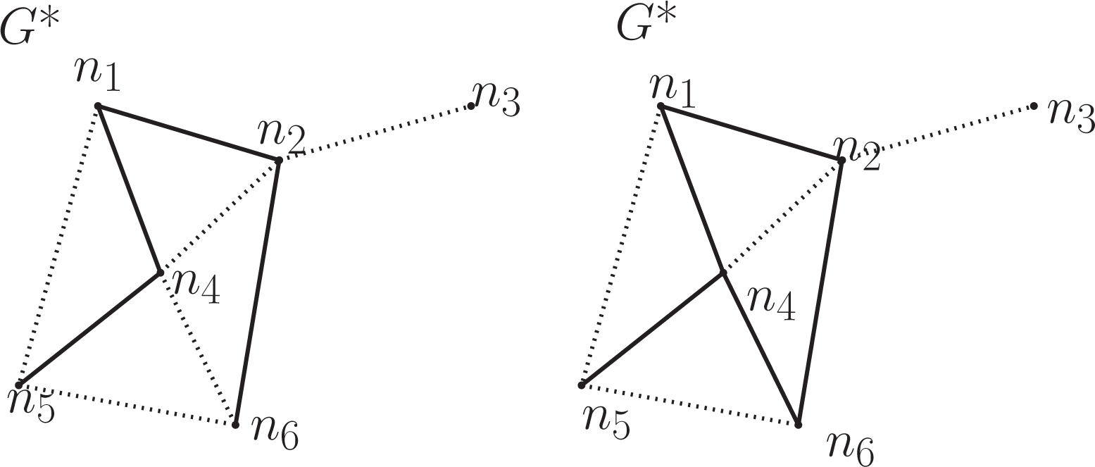
In the left figure, dotted lines present a cycle-removing edge cover of G*. In the right figure, dotted lines present an edge cover of G* that is not cycle-removing.

We prove the following statement:

Theorem 2

Consider a Voronoi diagram G such that G* is a connected graph with multiple nodes. $N_{min} \leq 2 | β^{*} |$ .

We present a proof of Theorem 2 by introducing Algorithm 3. Utilizing Algorithm 3, at most $2 | β^{*} |$ guards are positioned to block all cycles.

Consider a cycle C of the Voronoi diagram G. C will enclose a region that is a connected subgraph of G. We denote this subgraph as $G [C]$ . The dual graph of $G [C]$ will be denoted as $G^{*} [C]$ . The edges forming the cycle C come from the Voronoi cells that correspond to nodes on the boundary of the dual graph $G^{*} [C]$ . These boundary nodes of the dual graph are connected by edges of the dual graph $G^{*} [C]$ . We will prove lemmas which will lead to the proof of Theorem 2.

Lemma 5

If C encloses a single cell, then guards positioned by Algorithm 3 block C.

Proof

The dual graph $G^{*} [C]$ is one node of G*. This node will be covered by an edge in β*. Hence, an edge between this node and a node corresponding to a Voronoi cell outside of C will be chosen. Guards are then positioned on both ends of an edge of C and C is blocked. □

Lemma 6

If C encloses multiple cells, then guards positioned by Algorithm 3 block C.

Proof

Consider the dual graph G*. If an edge in β* connects a node that belongs to $G^{*} [C]$ with a node that does not belong to $G^{*} [C]$ , then similarly to the proof of Lemma 5, the cycle C must be blocked by guards positioned by Algorithm 3.

On the other hand, suppose the edges in β* that cover the nodes of $G^{*} [C]$ all belong to $G^{*} [C]$ . Then, consider the boundary nodes of $G^{*} [C]$ . Arbitrarily choose an edge between any two boundary nodes, then this edge corresponds to a Voronoi edge on G that intersects C. If this edge belongs to β*, since both ends of the corresponding Voronoi edge will be guarded, then at least one guard will be positioned on C to block C.

We now show that there exists at least one edge in β* that connects two boundary nodes of $G^{*} [C]$ . Suppose $G^{*} [C]$ does not contain a cycle, then all nodes in $G^{*} [C]$ are boundary nodes. Because these nodes need to be covered by β*, then at least one edge connecting two boundary nodes belongs to β*. Since $G^{*} [C]$ is a plane graph, if $G^{*} [C]$ contains a cycle, then its boundary must contain a cycle. Then, at least one edge between two boundary nodes must belong to β* to remove this boundary cycle. Therefore, we have shown that β* must contain an edge between boundary nodes of $G^{*} [C]$ . Hence, Algorithm 3 will deploy guards to block C. □

We next prove Theorem 2:

Proof

According to Lemmas 5 and 6, any cycle C in G will be blocked by Algorithm 3. Then, the minimum number of guards needed to block all cycles in G is not bigger than $2 | β^{*} |$ . Hence, $N_{min} \leq 2 | β^{*} |$ . □

A special case

We next consider the case in which G* is a tree and show that the number of guards needed can be significantly reduced. A typical environment in which G* is a tree graph is a corridor in a building. We have the following theorem.

Theorem 3

Consider the Voronoi diagram G whose dual graph G* is a tree. $N_{min} \leq | β^{*} |$ .

Since there is no cycle in the dual graph G* because of its tree structure, the minimum cycle-removing edge cover β* coincides with the minimum edge cover of G*. This is desirable considering computational complexity, since the minimum edge cover of G* can be calculated in polynomial time. The proof is based on Algorithm 4. We will show that Algorithm 4 removes all cycles in G.

Algorithm 4.

Guarding at most $| β^{*} |$ nodes in G.

Lemma 7

If C encloses a single cell, then guards positioned by Algorithm 4 block C.

The proof is similar to the proof for Lemma 5. One guard is enough to block the cycle C.

Lemma 8

Let C be a cycle in G enclosing at least two Voronoi cells V₁ and V₂. Suppose $G^{*} [C]$ is a tree graph. Moreover, let $e_{1, 2}$ denote the boundary edge shared between ∂V₁ and ∂V₂. Then, both end points of e_1,2 are on C.

Proof

Let n₁ and n₂ be the nodes of G* that correspond to V₁ and V₂, respectively. Because of the tree structure of G*, the edge connecting n₁ and n₂ is the only path between n₁ and n₂, since otherwise $G^{*} [C]$ will contain a cycle.

Suppose one end of e_1,2 is not on C. Denote this end point as E₁. E₁ must be inside the cycle C. According to the definition of a Voronoi vertex, there exist at least two Voronoi edges other than e_1,2 that share E₁ as an end point. If there are exactly two Voronoi edges other than e_1,2, then the two edges belong to one Voronoi cell, say V₃, that is adjacent to both V₁ and V₂. On the dual graph $G^{*} [C]$ , the three Voronoi cells will correspond to three nodes that form a cycle. If there are more than two Voronoi edges other than e_1,2, then each adjacent pair of edges will define one Voronoi cell that corresponds to a node on $G^{*} [C]$ . These nodes will form a path that connects n₁ and n₂, which then forms a cycle with the edge $n_{1} n_{2}$ on the dual graph $G^{*} [C]$ . This is illustrated in Figure 5. □

Figure 5.

The Voronoi vertex E₁ is inside C, and e_1,2 (the bold line) is the common edge shared by V₁ and V₂ that corresponds to the edge connecting n₁ and n₂ on the dual graph $G^{*} [C]$ to the left. Then, since there are edges other than e_1,2 meet E₁, there exists cells, such as V₃ and V₄, that form cycles with V₁ and V₂ on the dual graph.

Lemma 9

If C encloses multiple cells, then guards positioned by Algorithm 4 block C.

The proof of Lemma 9 is similar to the proof of Lemma 6, except Lemma 8 should be used to argue that the cycle C is blocked by guarding a single end node of $e_{i, j}$ .

Theorem 3 is then proved since Algorithm 4 removes all cycles in G.

The relationship between the number of guards required and the number of obstacles

We derive the relationship between N_min and the number of obstacles if there exists a perfect matching for G*.

Lemma 10

Consider a Voronoi diagram G modeling the environment W satisfying assumptions (1) and (2). Let M be the number of obstacles where the M th obstacle is the boundary obstacle. If a cycle-removing edge cover of G* is a perfect matching in G*, then $N_{min} \leq M - 1$ . Furthermore, if G* is a tree, then $N_{min} \leq \frac{M - 1}{2}$ .

Proof

Since the perfect matching is a minimum cycle-removing edge cover, we have $| β^{*} | = \frac{M - 1}{2}$ . Therefore, $N_{min} \leq M - 1$ follows utilizing Theorem 2. And if G* is a tree, then $N_{min} \leq \frac{M - 1}{2}$ follows from Theorem 3. □

Simulation results

Multi-robot exploration algorithms

Utilizing MATLAB simulations, we compare the performance of our multi-robot exploration algorithms with BE algorithms in the study by Kim et al.⁶ We consider the environment identical to the environment in the study by Kim et al.⁶ The obstacle boundaries are depicted with thick red curves in all figures. Along the trajectory of a robot, Voronoi vertices are shown as large dots. The robot speed is 10 distance units per unit time. To make the robot traverse a Voronoi edge, we use the controller of the work by Kim et al.⁶ We consider the case in which the robot’s sensor range is long enough to detect a blocked sector. Therefore, the robot does not move through a blocked sector.

Figure 6 shows the trajectory of one robot under BE algorithms in the study by Kim et al.⁶ Initially, the robot is at (2, 20). Also, the robot’s trajectory is shown with green circles.

Figure 6.

The Voronoi diagram constructed by BE algorithms. BE: boundary expansion.

In Figure 7, two robots build the Voronoi diagram in the environment that is identical to that in Figure 6. Initially, two robots are at (2, 20) and (2, 15), respectively. This implies that the initial enclosing boundaries B₀ built by two robots are identical. Moreover, the robots’ trajectories are shown with points and circles, respectively.

Figure 7.

Two robots building the Voronoi diagram under SCN algorithms. The initial enclosing boundaries built by two robots are identical. SCN: Simultaneous Cooperative Networking and exploration.

In Figure 8, two robots build the Voronoi diagram in the environment that is identical to that in Figure 6. Two robots’ initial locations are (2, 20) and (45, 2), respectively. Moreover, the trajectories of two robots are shown as points and circles, respectively.

Figure 8.

Two robots building the Voronoi diagram under SCN algorithms. SCN: Simultaneous Cooperative Networking and exploration.

We also simulated the case in which three robots construct the Voronoi diagram in the environment that is identical to that in Figure 6. Figure 9 shows three robots building the Voronoi diagram in the environment that is identical to that in Figure 6. Initially, three robots are at (2, 20), (20, 3), and (45, 2), respectively.

Figure 9.

Three robots building the Voronoi diagram under SCN algorithms. SCN: Simultaneous Cooperative Networking and exploration.

Table 2 shows the exploration time in the case where the number of deployed robots varies. As we increase the number of deployed robots, the exploration time decreases.

Table 2.

Exploration time as we vary N_v, the number of robots.

Metric	N _v = 1 (Figure 7)	N _v = 2 (Figure 8)	N _v = 2 (Figure 9)	N _v = 3 (Figure 10)
Exploration time (Time units)	63	47	18	13

Figure 10 shows both the Voronoi diagram D and obstacle environments with four circular obstacles. Thick red curves imply obstacle boundaries. Utilizing SCN algorithms, two robots build D. One robot starts from (2, 4), while another robot starts from (19, 6). See that D contains four cycles.

Figure 10.

The Voronoi diagram D and obstacle environments. D* is a line graph with four nodes. Deployed guards are depicted as two red dots.

Table 3 shows the exploration time as we vary the number of deployed robots. We simulated the case in which one robot, which starts from (2, 4), builds D utilizing BE algorithms in the study by Kim et al.⁶ Also, we simulated the case in which two robots, which start from (2, 4) and (19, 6), respectively, build D utilizing SCN algorithms. We further simulated the case in which three robots, which start from (2, 4), (19, 6), and (28, 5), respectively, build D utilizing SCN algorithms. As we increase the number of deployed robots, the exploration time decreases in general. However, in the case where we increase N_v from 2 to 3, the exploration time does not decrease anymore.

Table 3.

Exploration time as we vary N_v, the number of robots (D* is a line graph).

Metric	$N_{v} = 1$	$N_{v} = 2$	$N_{v} = 3$
Exploration time (Time units)	14	4	4

Intruder capture algorithm

Since we assume that every robot’s weapons are powerful enough to cover the width of a passage between obstacles, we can simplify our scenario such that a searcher and an intruder traverse Voronoi edges. In Figure 10, guards are depicted as large red dots. In the figure, two guards are located at two vertices in D, so that all cycles are blocked. D*, the dual graph of D, in Figure 10 is a line graph with four nodes. Thus, Algorithm 4 is used to deploy guards. Once two guards are located at two vertices, so that all cycles are blocked, then one free robot can chase one intruder at a time until every intruder is captured. Because of two guards, no intruder can run away from the free robot no matter how fast the intruder is. Our intruder capture algorithm works regardless of the number of worst-case intruders.

Recall D* is a line graph with four nodes. The minimum edge cover of this line graph is two. Thus, N_min is equal to or less than two utilizing Theorem 3. See that one guard cannot block all cycles in D. Thus, $N_{min} = 2$ for D in Figure 10.

Conclusions

The central idea of SCN algorithms is that each robot explores by gradually expanding the explored parts of the environment. At the same time, every robot deploys nodes and, as a result, a sensor network based on Voronoi diagrams is built. We prove that such a cooperative exploration results in efficient construction of the Voronoi diagram. Once the sensor network is completely constructed, this network can then be utilized by the robots to secure the environment. Guarding robots can be positioned at locations to ensure that no intruder can escape, while one free robot can capture every intruder one by one. In our future works, we will do experiments to verify the effectiveness of both our SCN algorithms and our intruder capture algorithm based on sensor networks.

Footnotes

Author’s note

All figures and tables are created by Jonghoek Kim.

Declaration of conflicting interests

The author(s) declared no potential conflicts of interest with respect to the research, authorship, and/or publication of this article.

Funding

The author(s) disclosed following financial support for the research, authorship, and/or publication of this article: This work was supported by the Hongik University new faculty research support fund.

References

Culler

Estrin

Srivastava

. Overview of sensor networks. IEEE Computer Magazine 2004; 37(8): 41–49.

Souryal

Geissbuehler

Miller

. Real-time deployment of multihop relays for range extension. In: Proceedings of the 5th international conference on mobile systems, applications and services (MobiSys 07), San Juan, Puerto Rico, 11–13 June 2007, pp. 85–98. New York, NY: ACM.

Liu

Xie

. Automatic and robust breadcrumb system deployment for indoor firefighter applications. In: Proceedings of the 8th international conference on mobile systems, applications, and services (MobiSys 10), San Francisco, California, USA, 15–18 June 2010, pp. 21–34. New York, NY: ACM.

Smith

Howard

McNew

. Multi-robot deployment and coordination with embedded graph grammars. Auton Robots 2009; 26(1): 79–98.

Kim

Zhang

Egerstedt

. Simultaneous cooperative exploration and networking based on Voronoi diagrams. In: Proceedings of IFAC workshop on networked robotics, Colorado, USA, pp. 1–6, 2009.

Kim

Zhang

Egerstedt

. A provably complete exploration strategy by constructing Voronoi diagrams. Auton Robots 2010; 29(3–4): 367–380.

Choset

Nagatani

. Topological simultaneous localization and mapping (SLAM): toward exact localization without explicit localization. IEEE Trans Rob Autom 2001; 17(2): 125–137.

Nagatani

Choset

. Toward robust sensor based exploration by constructing reduced generalized Voronoi graph. In: Proceedings IEEE/RSJ international conference on intelligent robots and systems, Kyongju, South Korea, 17–21 October 1999, pp. 1687–1692. USA: IEEE.

Rao

NSV

Stoltzfus

Iyengar

. A retraction method for learned navigation in unknown terrains for a circular robot. IEEE Trans Rob Autom 1991; 7(5): 699–707.

10.

Lavalle

. Planning Algorithms. England: Cambridge University Press, 2006.

11.

Pimenta

CAL

Schwager

Lindsey

. Simultaneous coverage and tracking (SCAT) of moving targets with robot networks. In: Algorithmic Foundation of Robotics VIII: Springer Tracts in Advanced Robotics (eds Chirikjian

Choset

Morales

.), Berlin, 7–9 December 2008, pp. 85–99. Heidelberg: Springer.

12.

Cortés

Martnez

Karatas

. Coverage control for mobile sensing networks. IEEE Trans Rob Autom 2004; 20(2): 243–255.

13.

Cunningham

Paluri

Dellaert

. DDF-SAM: fully distributed slam using constrained factor graphs. In: IEEE/RSJ international conference on intelligent robots and systems (IROS), Taipei, Taiwan, 18–22 October 2010, pp. 3025–3030. Taiwan: IEEE.

14.

Howard

Mataric

Sukhatme

. Relaxation on a mesh: a formalism for generalized localization. In: Proceedings 2001 IEEE/RSJ international conference on intelligent robots and systems, Maui, HI, USA, 29 October–3 November 2001, pp. 1055–1060. USA: IEEE.

15.

Mao

Fidan

Anderson

ODB

. Wireless sensor network localization techniques. Comput Netw 2007; 51(10): 2529–2553.

16.

Priyantha

Balakrishnan

Demaine

. Anchor-free distributed localization in sensor networks. In: Proceedings of the first international conference on embedded networked sensor system, Los Angeles, CA, USA, 5–7 November 2003, pp. 340–341. New York, NY: ACM.

17.

Jiang

Lin

. ALRD: AoA localization with RSSI differences of directional antennas for wireless sensor networks. Int J Distrib Sens Netw 2013; 9: 529489. doi: 10.1155/2013/529489.

18.

Han

Duong

. Localization algorithms of wireless sensor networks: a survey. Telecommunication Syst 2013; 52(4): 2419–2436.

19.

Cheng

Zhang

. A survey of localization in wireless sensor network. Int J Distrib Sens Netw 2012; 8: 962523. doi: 10.1155/2012/962523.

20.

Niculescu

Nath

. Ad hoc positioning system (APS) using AOA. In: Twenty-second annual joint conference of the IEEE computer and communications, San Francisco, CA, 30 March–3 April 2003, pp. 1734–1743. USA: IEEE.

21.

Thrun

Montemerlo

Thrun

. The graph slam algorithm with applications to large-scale mapping of urban structures. Int J Rob Res 2006; 25(5–6): 403–429.

22.

Parsons

. Pursuit-evasion in a graph. In: Theory and applications of graphs—Lecture notes in mathematics. Germany: Springer-Verlag, 1978, 642: 426–441.

23.

Kolling

Carpin

. Pursuit-evasion on trees by robot teams. IEEE Trans Robot 2010; 26(1): 32–47.

24.

Seymour

Thomas

. Graph searching and a min-max theorem for tree-width. J Comb Theory B 1993; 58: 22–33.

25.

Richerby

Thilikos

. Graph searching in a crime wave. SIAM J Discrete Math 2009; 23(1): 349–368.

26.

Kim

. Cooperative exploration and protection of a workspace assisted by information networks. Ann Math Artif Intell 2014; 70(3): 203–220.

27.

Kim

. Cooperative exploration and networking while preserving collision avoidance. IEEE Trans Cybern 2016; 47(12): 4038–4048.

28.

Kim

. Capturing intruders based on Voronoi diagrams assisted by information networks. Int J Adv Robot Systems 2017; 14(1): 1–8. Article ID: 962523.

29.

Megiddo

Hakimi

Garey

. The complexity of searching a graph. J ACM 1988; 35(1): 18–44.

30.

Kolling

Carpin

. The graph-clear problem: definition, theoretical properties and its connections to multirobot aided surveillance. In: Proceedings of the 2007 IEEE/RSJ international conference on intelligent robots and systems, San Diego, CA, 29 Oct–2 Nov 2007, pp. 1003–1008. USA: IEEE.

31.

Lapaugh

. Recontamination does not help to search a graph. J ACM 1993; 40(2): 224–245.

32.

Fomin

Fraigniaud

Nisse

. Nondeterministic graph searching: from pathwidth to treewidth. Algorithmica 2009; 53(3): 358–373.

33.

Barriére

Flocchini

Santoro

. Capture of an intruder by mobile agents. In: Proceedings of the fourteenth annual ACM symposium on parallel algorithms and architectures, Winnipeg, MB, 11–13 August 2002, pp. 200–209. Canada: ACM.

34.

Fomin

Thilikos

. An annotated bibliography on guaranteed graph searching. Theor Comput Sci 2008; 399(3): 236–245.

35.

Makedon

Sudborough

. On minimizing width in linear layouts. Discrete Appl Math 1989; 23(3): 243–265.

36.

Kirousis

Papadimitriou

. Interval graphs and searching. Discrete Math 1985; 55(2): 181–184.

37.

Kirousis

Papadimitriou

. Searching and pebbling. Theor Comput Sci 1986; 42(2): 205–218.

38.

Bienstock

Paul

. Monotonicity in graph searching. J Algorithms 1991; 12(2): 239–245.

39.

Nick

Lefieris

Dimitrios

. Fugutive-search games on graphs and related parameters. Theoretical Comput Sci 1997; 172: 233–254.

40.

Chung

Hollinger

Isler

. Search and pursuit-evasion in mobile robotics. Auton Robot 2011; 31: 299–316.

41.

Kolling

Carpin

. Extracting surveillance graphs from robot maps. In: Proceedings of intelligent robots and systems, Nice, France, 22–26 September 2008, pp. 2323–2328. IEEE.

42.

Borie

Tovey

Koenig

. Algorithms and complexity results for graph-based pursuit evasion. Auton Robot 2011; 31(4): 317.

43.

Douglas

. Introduction to graph theory. 2nd ed. Illinois, USA: Prentice Hall, 2001.

44.

Edmonds

. Paths, trees, and flowers. Canadian J Math 1965; 17: 449–467.

45.

Kolmogorov

Blossom V: a new implementation of a minimum cost perfect matching algorithm. Math Prog Comput 2009; 1(1): 43–67.

46.

Aurenhammer

. Voronoi diagrams-a survey of a fundamental geometric data structure. ACM Comput Surveys 1991; 23(3): 345–405.

47.

Klein

Concrete and abstract Voronoi diagrams. Germany: Springer, 1990.

48.

Choset

Burdick

. Sensor-based exploration: the hierarchical generalized Voronoi diagram. Int J Robot Res 2000; 19(2): 96–125.

49.

Bhattacharya

Gavrilova

. Roadmap-based path planning - using the Voronoi diagram for a clearance-based shortest path. IEEE Robot Autom Mag 2008; 15(2): 58–66.

Workspace exploration and protection with multiple robots assisted by sensor networks

Abstract

Keywords

Introduction

Related works

Preliminaries and background

Graphs

The environment and its Voronoi diagram

Assumption 1

Assumption 2

BE algorithms

Exploring while networking

Boundary merge

Complexity analysis

Performance analysis

Lemma 1

Theorem 1

Proof

Securing the environment

Clearing a tree graph

Lemma 2

Lemma 3

Proof

Clearing a Voronoi diagram

Lemma 4

Theorem 2

Lemma 5

Proof

Lemma 6

Proof

Proof

A special case

Theorem 3

Lemma 7

Lemma 8

Proof

Lemma 9

The relationship between the number of guards required and the number of obstacles

Lemma 10

Proof

Simulation results

Multi-robot exploration algorithms

Intruder capture algorithm

Conclusions

Footnotes

Author’s note

Declaration of conflicting interests

Funding

References