Sage Journals: Discover world-class research

Abstract

This paper presents a chaotic motion path planner based on a Logistic Map (SCLCP) for an autonomous mobile robot to cover an unknown terrain randomly, namely entirely, unpredictably and evenly. The path planner has been improved by arcsine and arccosine transformation. A motion path planner based only on the Logistic Chaotic Map (LCP) can show chaotic behaviour, which possesses the chaotic characteristics of topological transitivity and unpredictability, but lacks better evenness. Therefore, the arcsine and arccosine transformations are used to enhance the randomness of LCP. The randomness of the followed path planner, LCP, the improved path planner SCLCP and the commonly used Random Path Planner (RP) are discussed and compared under different sets of initial conditions and different iteration rounds. Simulation results confirm that a better evenness index of SCLCP can be obtained with regard to previous works.

Keywords

Autonomous Mobile Robot SCLCP Evenness Chaos Arcsine and Arccosine Transformation

1. Introduction

The subject of this research is an autonomous mobile robot that can be used as patrol robot or robot for cleaning in closed areas. This scanning does not demand a planning trajectory of the autonomous mobile robot in this schema that knows the workspace and obstacles. It does, however, require the robot path to cover every part of the workspace. One robot with these characteristics is a chaotic autonomous mobile robot. The main characteristics of the chaotic systems are the topological transitivity and the sensitive dependence on initial conditions [1]. Due to topological transitivity, the chaotic autonomous mobile robot is guaranteed to scan the whole connected workspace. The sensitive dependence on initial conditions is a desirable characteristic for patrol robots, since the trajectory of the chaotic autonomous mobile robot is very unpredictable [2 –4]. The interaction between autonomous mobile robotics and chaos theory has been studied only recently [5 –7]. The key problem of this research is how to impart the chaotic motion behaviour on to the autonomous mobile robot. Some related work has been done. For instance, the integration between the robot motion system and a chaotic system, the Arnold dynamical system, is used to impart chaotic behaviour to a robot in [8]. The same principle of systems integration is adopted to generate the random motion for complete coverage path planning of the mobile robot in [3]. In [9], an open-loop control approach is proposed to produce an unpredictable trajectory so that the state variables of the Lorenz chaotic system are used to command the velocities of the robot's wheels. Other known chaotic systems, such as a Standard or Taylor–Chirikov map and a Chua circuit [10] have been used.

However, most of the above research has regarded chaotic systems as totally default random ones. This ignorance can bring about uneven patrolling terrain in some circumstances. In this paper, we propose an improved chaotic path planner SCLCP for an autonomous mobile robot with a chaotic change of the angle. We suggest that the robot's angle should be changed using rule of Logistic chaotic map and the chaotic equation has been improved to obtain good randomness characteristics to ensure that the chaotic trajectory cover the entire areas of patrolling more evenly. In order to reveal the superiority of the chaotic path planner, the common used random path planner RP, is also discussed for contrast. Simulation results illustrate the usefulness of the proposed path planner.

The paper is organized as follows. Section 2 presents a chaotic path planner LCP and its uniformity test based on the logistic map. Another commonly used random path planner RP is discussed in Section 3. Section 4 assumes arcsine and arccosine transformations to obtain an improved path planner SCLCP based on LCP. χ² test of numerical analysis is assumed in Section 5 to test the evenness of path planner LCP, RP and SCLCP. Section 6 provides numerical simulations of SCLCP. Conclusions are drawn in Section 7.

2. Chaotic Path Planner LCP with Logistic Map

In this paper an autonomous mobile robot moves with a constant velocity and is steered by the variables of a logistic map. By interval mapping, the angle of the robot has the same chaotic variation characteristics as the logistic map.

2.1 Discussion of the Logistic bifurcation map

A logistic map is the deterministic, discrete-time dynamical system of an iterative map. The equation can be described in the form of:

x_{n + 1} = μ x_{n} (1 - x_{n})

(1)

Where μ∈ [0,4], k = 0,1, …, n is the discrete time and x₀,x₁, …, x_n are the states of the system at different instants in time. Starting from the initial state x₀, the repeated iteration of Equation (1) gives rise to a fully deterministic series of states known as an orbit. It is used as a model for a chaos generator. The relative simplicity of the Logistic map makes it an excellent point of entry into a consideration of the concept of chaos. Figure 1 describes the orbit of the Logistic bifurcation map when the parameter μ changes among the range [0,-4] while the initial condition x₀ remains constant. Figure 1 (a) and (b) draw the iterative trajectories under different initial condition x₀.

Figure 1.

Orbit of the Logistic bifurcation map

Though the initial condition x₀ is different, the orbits all show similar chaos characteristics when parameter μ changes among the range (3.57-4]. In fact, all values of x₀ among (0-1) have these properties. Especially Figure 1 shows that when μ converges to 4, the {x_k} orbits become increasingly chaotic and demonstrate a pseudorandom and uniform distribution among the range (0-1) [11]. Slight variations in x₀ result in dramatically different orbits, an important characteristic of chaos. So we use the Logistic equation (2) as a random number generator.

x_{n + 1} = 4 x_{n} (1 - x_{n})

(2)

2.2 Integrated system (LCP) of the Logistic map and the robot

The autonomous mobile robot considered in this work is a typical differential motion with two degrees of freedom, composed by two active, parallel and independent wheels, and a third passive wheel with an exclusive equilibrium function [12]. The active wheels are independently controlled on velocity and sense of turning. The sensors provide short-range distances to obstacles. The resultant motion is described in terms of linear velocity v and direction θ. These equations constitute a nonholonomic dynamical system. The robot kinematics model is described by (3), where x and y identify the robot position and θ is the orientation.

{\begin{cases} \dot{x} = v \cos θ \\ \dot{y} = v \sin θ \\ \dot{θ} = ω \end{cases}

(3)

The discrete form of the Equation (3) is:

{\begin{cases} x_{n + 1} \approx x_{n} + h v \cos θ_{n} \\ y_{n + 1} \approx y_{n} + h v \cos θ_{n} \\ θ_{n + 1} \approx θ_{n} + h ω_{n} \end{cases}

(4)

Where h is a sufficiently small step.

The variation range scope of the robot orientation angle θ_n is $(- \frac{π}{2}, + \frac{π}{2})$ . While x_n is in the logistic map located in (0-1). In order to integrate the logistic map into the path planner of autonomous mobile robot, we define the following transformation:

{\begin{cases} θ_{n} = π x_{n} - π / 2 \\ x_{n + 1} = 4 x_{n} (1 - x_{n}) \end{cases}

(5)

Then the discrete model of the robot is:

{\begin{cases} x_{n + 1} \approx x_{n} + h v \cos θ_{n} \\ y_{n + 1} \approx y_{n} + h v \sin θ_{n} \\ θ_{n} = π x_{n} - \frac{π}{2} \\ x_{n + 1} \approx 4 x_{n} (1 - x_{n}) \end{cases}

(6)

Now, the angle θ_n of the robot is calculated iteratively depending on equation (6). So the robot path planner designed as equation (6) possesses the chaotic characteristics. Here we defined the planner as LCP (Logistic Control Planner).

2.3 Uniformity Test of LCP

Equation (6) assumes that each autonomous mobile robot works in a smooth state space without boundaries. However, real autonomous mobile robots move in space with boundaries like the walls of the surfaces of obstacles. To avoid obstacles, we can adopt the mirror mapping approach as shown in [7]. Here, we do not think about obstacle influence on the path planner.

Because θ_n and x_n own the same chaotic characteristics and random distribution characteristics according to Equation (5), here we only discuss the random distribution characteristics of x_n for convenience and then map it to θ_n space.

The terrain covering can be judged through a performance index. This index can be defined using terrain division on square unit cells and computing the visited cells percentage after the robot location planning [12 –14]. Here the uniformity test of LCP is carried through by the evenness computation among each equal interval. In this section we obtain the chaotic state variables x_n of LCP and measure the probability density of x_n under different initial conditions and different iteration rounds. x_n sequences are divided into ten same length sub- intervals between 0-1, namely 0-0.1, 0.1-0.2, … and 0.9-1 respectively and the numbers k(m) (m = 1, …, 10) that lie within each sub-interval are counted and displayed. A good pseudorandom sequence should have uniformity of unit intervals.

Four sequences are generated with different sets of initial conditions and different iteration rounds. Each element of the sequences can be changed to the robot position according to Equation (3). Their uniformity distribution and the numbers k(m) are described in Figure 2 - Figure 5.

Figure 2.

Terrain covering circumstance under x₀ = 0.1, n=1000; (a) Uniformity distribution in the covering terrain (b) k(m) that lies within each sub-interval

Figure 3.

Terrain covering circumstance under x₀ = 0.7, n=1000; (a) Uniformity distribution in the covering terrain (b) k(m) that lies within each sub-interval

Figure 4.

Terrain covering circumstance under x₀ = 0.1, n=10000; (a) Uniformity distribution in the covering terrain (b) k(m) that lies within each sub-interval

Figure 5.

Terrain covering circumstance under x₀ = 0.7, n=10000; (a) Uniformity distribution in the covering terrain (b) k(m) that lies within each sub-interval

It is obvious that the pseudorandom sequences of LCP are distributed unevenly in the scanning working area. The distribution features demonstrate characteristics of two edges being thick and the middle being thin in the covering space. This has little relation with the initial conditions and iteration rounds. The chaos sequence of LCP can meet our needs for this general case. In order to obtain a better distribution uniform, the performance of the presented LCP should be enhanced.

3. Randomness Discussion of RP

Another commonly used method for scanning unknown workspace with barriers without a planning trajectory to use an autonomous mobile robot with a random change of the angle. Here we call this random path planner a RP for an autonomous mobile robot. We need to discuss the uniform distribution of the sequence generated by RP compared with LCP to reveal the superiority of the chaotic path planner. The simulation environment and the constant velocity of the robot are the same as those of the previous work.

A Linear Congruential Generator (LCG) represents one of the oldest and best-known pseudorandom number generator algorithms. LCG is fast and requires minimal memory (typically 32 or 64 bits) to retain state. The generator is defined by the recurrence relation:

{\begin{cases} x_{n} = (a x_{n - 1} + c) (\mod M) \\ r_{n} = x_{n} / M \\ i n i t i a l s t a t e x_{0} \end{cases} (n = 1, 2, ...)

(7)

Where x_n is the sequence of the pseudorandom values and a, c and m are integer constants that specify the generator. The LCG defined above has a full period if and only if the parameters c, m, and a have been a suitable chosen value. Here we use LCG as the RP sequence generator. In order to compare the uniform distribution of a standard random signal of RP with the mentioned method LCP, the same analysis method is assumed.

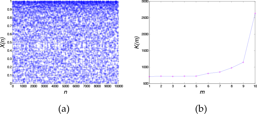
Figure 6 and Figure 7 show that the distribution feature has a close relationship with the iteration rounds of the random function. The greater the rounds of iteration, the better the performance of the uniform distribution behaves. This shows that the RP can meet some needs of certain application when the iteration rounds are large enough.

Figure 6.

Terrain covering circumstance at n=1000 (a) Uniformity distribution in the covering terrain (b) k(m) that lies within each sub-interval

Figure 7.

Terrain covering circumstance at n=10000; (a) Uniformity distribution in the covering terrain (b) k(m) that lies within each sub-interval

4. Improved Path Planner SCLCP

Chaotic systems have the property of being deterministic in microscopic space and behave randomly, when observed in a coarse-grained state-space. The sensitivity of chaotic maps to initial conditions makes them optimum candidates to relate minimal critical information about the input, in the output sequence. Their iterative nature makes them quickly computable and able to produce binary sequences with extremely long cycle lengths. Therefore, the chaotic scan is stochastically superior to the scan by randomness to yield a favourable nature for a patrol robot if given the best adjusting parameters.

From Section 3 we know that the sequences distribution of LCP demonstrates characteristics with two edges that are thick and a thin middle. Therefore, the optimization goal of LCP is to be able to average the distribution of the two edges. Arcsine and arccosine transformations have been assumed for x_n sequence generated by LCP and their contribution to the transformation are discussed respectively. First only the arcsine transformation effect is tested:

x_{n} = \frac{2 \arcsin x_{n}}{π}

(8)

The distribution characteristics are shown in Figure 8. Figure 8 shows that the arcsine transformation smoothes the bigger edge distribution.

Figure 8.

Terrain covering circumstance under x₀ = 0.1, n=10000 using arcsine transformation; (a) Uniformity distribution in the covering terrain (b) k(m) that lies within each sub-interval

In a similar way, the arccosine transformation is taken:

x_{n} = \frac{2 \arccos x_{n}}{π}

(9)

Figure 9 shows that the transformation smoothes the smaller edge distribution. So if the arcsine and arccosine transformation are combined, the whole distribution characteristics of LCP could be enhanced. We call this improved LCP path planner SCLCP.

Figure 9.

Terrain covering circumstance under x₀ = 0.1, n=10000 using arccosine transformation; (a) Uniformity distribution in the covering terrain (b) k(m) that lies within each sub-interval

x_{n} = {\begin{cases} \frac{2 \arccos x_{n}}{π} 0 < x_{i} \leq 0.5 \\ \frac{2 \arcsin x_{n}}{π} 0.5 < x_{i} < 1 \end{cases}

(10)

Figure 10 shows the transformation effect. The chaotic random attributes have been changed obviously and the amount k(m) of each region is uniform and has no significant change.

Figure 10.

Terrain covering circumstance under x0 = 0.1, n=10000 of SCLCP; (a) Uniformity distribution in the covering terrain (b) k(m) that lies within each sub-interval

5. Numerical Analysis

We have discussed the x_n sequence's random characteristics of LCP, RP and SCLCP through simulation and graphics qualitatively. They demonstrate the difference between characteristics significantly seen from the results. The improved SCLCP produces better evenness than other path planner. Now we want to further discuss their diversity quantitatively, mainly by frequency tests. The methods test whether the diversity between the real frequency and the theoretical one that the random sequences distribute in the subinterval is significant or not. The two common frequency test methods are the K-S (Kolmogorov-Smirnov) test and χ² test. Here the χ² test is assumed [15].

The main point of the χ² test is to divide x_n sequences into k same length subintervals between 0 and 1 and examine the diversity between the real frequency and the theoretical one of the random sequence's distribution in the subinterval. Define the real frequency of the ith subinterval random data as n_i and the corresponding theoretical frequency of this subinterval is defined as m_i. Here m_i =N/k, where N is the total random sequences number. Statistic value χ² is constructed:

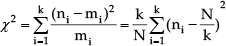
χ^{2} = \sum_{i = 1}^{k} \frac{{(n_{i} - m_{i})}^{2}}{m_{i}} = \frac{k}{N} {\sum_{i = 1}^{k} (n_{i} - \frac{N}{k})}^{2}

(11)

When N is big enough, the χ² value approximately obeys the distribution of the degree of freedom k-1. A critical value α is defined for the theoretical distribution. The significance level of the tests is commonly set to α = 0.01 ~ 0.05. When α is given a certain value, a critical value χ_α²(k-1) can be looked up from the table [16]. If χ² > χ_α²(k-1), the hypothesis for randomness evenness is rejected.

The test procedure of χ² is as follows.

Divide x_n sequences into k same length subintervals between 0 and 1

Count the total number n_i and calculate theoretical frequency m_i

Calculate χ² according to Equation (11)

Look up the critical value χ_α²(k-1) from the χ² table according to the given value α and degrees of freedom k-1

Compare value χ² with the critical value χ_α²(k-1), and determine whether to accept it or not.

At the same time, the quality of various path planners can be compared by the calculated results of χ². The smaller χ² is, the better the evenness is. χ² values of x_n sequences for the above mentioned path planners, LCP, RP and SCLCP have been calculated and tested. The results are listed in Table 1. Here, where α = 0.05, the critical value is 16.919 and the rejection region is {χ² ≥ χ_α²(k-1)}.

Table 1.

χ² test for pseudorandom number x_n sequences

Path Planner	x_n	χ ²	Declaration
LCP	Figure 3	287.8	reject
RP (1)	Figure 6	17.73	reject
RP (2)	Figure 7	4.315	accept
SCLCP	Figure 10	0.8402	accept

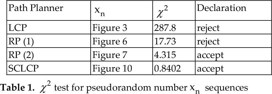
Values in the third column in Table 1 are the χ² test results. Compared with the critical value 16.919, 287.8 for LCP and 17.73 for RP (1) are larger and can't pass the evenness test. While RP (2) and SCLCP can pass the test with smaller values than 16.919 and have better evenness characteristics. For the same path planner RP, circumstance RP (2) has a greater number of iteration rounds than RP (1), so it has a better evenness performance. The quality sort of the above path planners is: SCLCP>RP(2)>RP(1)>LCP.

6. Numerical Simulations

To test our mobile robot patrolling approach, we have simulated the robot kinematic motion, applying the improved SCLCP discussed in this paper. Since we would like to use the robot in wandering around an area without maps, the chaotic trajectory should cover the entire area of patrolling as often as possible. A performance criteria, namely the performance index K, is considered to evaluate the coverage rate of the chaotic mobile robot. The index K represents a ratio of areas that the trajectory passes through or used (A_u), over the total working area (A_t),

K = \frac{A_{u}}{A_{t}}

(12)

For simplicity, an area of 1×1 is used as a workspace coverage trajectory in a computer simulation. The area can be divided into M×M grids to calculate index K. In this paper M=100. Initially, all grids are assigned the value 0. When the trajectory passes through the grid, the value is modified to one. We count the number of ones as A_u and the total grids number as A_t, A_t = M×M. Then index K can be counted according to the Equation (12).

By numerically simulating the map equations, we can analyse the properties of terrain coverage considering the basic mission requirements for fast terrain scanning. In the simulation environment, the obstacles number, position and size and the robot position and size, can be set up randomly. In the simulation environment shown in Figure 11, the solid blue circle shows the robot, the solid black circles are obstacles and the cyan curves show the planned trajectory. The initial conditions are established and the program is set to run N iterations. We can see that SCLCP can completely cover the considered terrain. The resultant SCLCP in two dimensions at iteration N=200, N=15000 are depicted in Figure 11.

Figure 11.

Numerical simulations of SCLCP

For N=15000, the performance index K has exceeded 99%, not including the grids which are occupied by the obstacles and are within the danger area near the obstacles and area edges. The unimproved chaotic path planner LCP needs more than 20000 iterations to obtain the same performance. While the random path planner RP needs about 16000 to do the same work.

7. Conclusion

In this paper, we have proposed an improved chaotic path planner SCLCP for an autonomous mobile robot, which implies a robot with a path planner that guarantees its chaotic motion. The Logistic equation, which is known to show the chaotic dynamics, is integrated into the autonomous mobile robot. Furthermore arcsine and arccosine transformations are used to enhance the evenness of the planner. The randomness of path planners are discussed and compared qualitatively and quantitatively. The improved path planner SCLCP has the following advantages.

It still guarantees the chaotic characteristics of topological transitivity and the sensitive dependence on initial conditions to meet the requirement of the patrolling task for an autonomous mobile robot

The evenness of the whole visiting workspace has been improved. It can generate an improved performance for complete coverage compared to LCP and RP

It has the property of being deterministic in a microscopic space and behaves randomly. Its randomness characteristics are relatively stable so it can be controlled by the designer's own compared with the randomness of path planner RP

The method is simple and effective. Its iterative nature makes it quick to computable and the robot can quickly obtain the controlling parameters and visit the workspace rapidly.

In future work we will further discuss other randomness characteristics, such as an independence test, a parameter test etc. of SCLCP and more research will be done in a real environment to test and improve the performances of the path planner.

Footnotes

8. Acknowledgments

This work is supported by the National Natural Science Foundation of China (No.61075091), The State Key Program of National Natural Science of China (No.61233014); National Natural Science Foundation for Young Scholars of China (No.61105100), Higher Educational Science and Technology Program of Shandong Province, China (No. J13LN27), and Shandong Province Natural Science Fund (No. ZR2010FL003).

References

Hasselblatt

and Katok

(2003), A first Course in Dynamics: With a Panorama of Recent Developments, Cambridge University Press, Cambridge.

Volos

C. K.

Kyprianidisb

I. M.

and Stouboulos

I. N.

(2012), A Chaotic Path Planning Generator for Autonomous Mobile Robots. Robotics and Autonomous Systems, 60 (4): 651–656.

Zhu

A.L.

and Leung

(2007). Cooperation Random Mobile Robots Based on Chaos Synchronization. Proceedings of International Conference on Mechatronics, 2007: 1–5.

Fallahi

and Leung

(2010). A Cooperative Mobile Robot Task Assignment and Coverage Planning Based on Chaos Synchronization. International Journal of Bifurcation and Chaos, 20 (1): 161–176.

Islam

and Murase

(2005). Chaotic Dynamics of a Behavior-based Miniature Mobile Robot: Effects of Environment and Control Structure. Neural Networks, 18 (2): 123–144.

Fahmy

A. A.

(2012), Chaotic Mobile Robot Workspace Coverage Enhancement. Journal of Automation, Mobile Robotics & Intelligent Systems, 6 (1): 33–38.

Kewlani

and Iagnemma

(2009), A Multi-Element Generalized Polynomial Chaos Approach to Analysis of Mobile Robot Dynamics under Uncertainty. IEEE/RSJ International Conference on Intelligent Robots and Systems: 1177–1182.

Nakamur

and Sekiguchi

(2001), The Chaotic Mobile Robot. IEEE Transaction on Robotics and Automation, 17 (6): 898–904.

Martins-Filho

L. S.

Machada

R. F.

Rocha

(2004), Commanding Mobile Robots with Chaos. In ABCM Symposium Series in Mechatronics, 1: 40–46.

10.

Sooraksa

Klomkarn

(2010). No-CPU Chaotic Robots: from Classroom to Commerce. IEEE Circuits and Systems Magazine, 10: 46–53.

11.

Peitgen

H. O.

Jürgens

and Saupe

(2004), Chaos and Fractals: New Frontiers of Science, Springer.

12.

Martins-Filho

L. M.

and Macau

E. E. N.

(2007), Patrol Mobile Robots and Chaotic Trajectories, Mathematical Problems in Engieering, Vol. 2007.

13.

Volos

C. K.

Kyprianidis

I. M.

and Stouboulos

I. N.

(2012), Motion Control of Robots Using a Chaotic Truly Random Bits Generator, Journal of Engineering Science and Technology Review, 5 (2): 6–11.

14.

Choset

(2006), Coverage for robotics-a survey of recent results, Annals of Mathematics and Artificial Intelligence, 31:113–126.

15.

Gao

X.H.

(1995), Statistical Computing, Peking University Press, China.

16.

Chen

X.L.

Shi

Q.SH.

and Deng

X.W.

(2011), Probability Theory and Mathematical Statistics The second Edition, Southeast University Press.