
Abstract
Abstract When operating autonomous unmanned aerial vehicles (UAVs) in real environments it is necessary to deal with the effects of wind that causes the aircraft to drift in a certain direction. In such conditions it is hard or even impossible for UAVs with a bounded turning rate to follow certain trajectories. We designed a method based on an Accelerated A* algorithm that allows the trajectory planner to take the wind effects into account and to generate states that are reachable by UAV. This method was tested on hardware UAV and the reachability of its generated trajectories was compared to the trajectories computed by the original Accelerated A*.
1. Introduction
This paper addresses the problem of three-dimensional trajectory path planning for UAVs with a bounded turning rate in the presence of constant wind, obstacles and other aircraft. To represent the motion dynamics of airplane-like UAVs, we apply constraints on flight manoeuvres and restrictions on the smoothness of the trajectory (trajectory and its first derivation are continuous).
In real environments UAVs are significantly susceptible to being drifted by wind. Particularly, aircraft with a bounded turning rate require different turning radii depending on the flight direction relative to the wind vector. For a successful and precise execution of a planned trajectory, the trajectory has to reflect the physical capabilities of the aircraft and the assumed impact of wind.
In this paper we present an approach based on an Accelerated A* (AA*) algorithm [11] for collision-free path planning in an environment with no-flight zones and other aircraft, which is capable of generating physically satisfiable plans in the presence of constant wind. The AA* algorithm was chosen because it is both complete and optimal and thanks to adaptive sampling it is fast even for large environments with a high number of obstacles.
A*-like algorithms are primarily intended to be used in fully observable deterministic environments. Real environments are non-deterministic, however we assume that the UAV has a GPS receiver to correct its position estimation and minimize the effects of non-deterministic actions. We also assume a prior knowledge of a map of the environment with obstacles defined as no-flight zones, thus considering the environment fully observable.
Our method has been successfully deployed and tested on a real fixed-wing UAV using Kestrel autopilot with significantly better results than those achieved by regular AA* algorithms in terms of plan execution precision.
The paper is organized as follows. In the following section we summarize related work dealing with path planning and the effects of wind. In Section 3 we describe the AA* algorithm our work is based on. Our modified version of the AA* algorithm is introduced in Section 4. In Section 5 we present the results we achieved and Section 6 concludes the paper.
2. Related work
The area of UAVs' trajectory planning has been the subject of many research works over the past several years. Numerous methods for flight trajectory planning in no-wind cases have been proposed. There are algorithms based on randomness, e.g., random-walk [3], rapidly exploring random trees (RRT) [8] or randomized potential fields [2]. These methods are fast but they are still based on random sampling and generally cannot find optimal solutions with respect to given criteria.
There are also algorithms computing optimal solutions that exploit pre-computed structures for a given environment definition – potential field path planning [7], vector field methods [9] or the 3D Field D* algorithm [4]. However, these approaches need to recalculate their inner data structures every time the environment changes.
The impact of wind effects on trajectory planning was dealt with in [10] by iteratively solving a no wind case problem with a moving virtual target, or in [13] by generating candidates of smooth (continuous curvature) time-optimal paths between initial and final points in the plane. These approaches search only for a horizontal plan between the start and final configuration and do not take possible obstacles into account. Cobano et al. [5] used a genetic algorithm and the Monte-Carlo method to deal with wind effects and to solve collisions noncooperatively. However this is also a randomized approach that does not have to find optimal solution and is not suitable for cooperative collision avoidance methods.
Our approach is based on an AA* algorithm, which can, thanks to adaptive sampling, efficiently (in a short time) find optimal paths in three dimensional environments with obstacles. The algorithm was modified to take the effects of wind and the limitations of the aircraft into account and is suitable for cooperative collision avoidance.
3. Accelerated A*
Accelerated A* (AA*) is a modified version of the A* algorithm presented in [11] that overcomes the trade-off between search speed (efficiency) and search precision by using an adaptive sampling mechanism. The algorithm generates samples of state space using elementary flight manoeuvres where the length of the manoeuvres is given by the aircraft's distance to the nearest obstacle - the further the obstacle the sparser the sampling and vice versa (see Figure 1). Search precision is defined by a minimal sampling step.

Example of the adaptive sampling. Taken from [11].
The AA* algorithm finds optimal trajectories only with respect to the sampling used. However, thanks to the use of an adaptive sampling mechanism (dependent on the distance to the closest obstacle), AA* is in this domain typically faster than the original A* algorithm with uniform sampling, which allows the use of a much smaller minimal sampling step while preserving the low computational requirements.
Manoeuvres that define the sampling and correspond to the aircraft's elementary actions are straight elements that are given by the start configuration and length, horizontal turn and vertical turn that are defined by the turning radius, arc angle and turn direction - left or right, respectively, and up or down.
The algorithm works in the same way as regular A*. It removes the best state from the OPEN list and if it can be directly connected with the goal state, it smoothes the found path by application of Dubins manoeuvres [6] when possible and returns the plan. Otherwise, it expands the current state by applying actions represented by the flight manoeuvres, estimates the new position and new sampling, checks the presence of this new state in the CLOSED list and checks the validity of the element, counts heuristics using Dubins curves and inserts the new state into the OPEN list. The sampling of continuous space can generate an infinite number of states where none are exactly the same. To prevent this, two states are considered equal if their Euclidean distance and their direction vectors differ less than a specified value given by the sampling parameterization used.
4. Modified AA* for planning in wind
Wind influences the minimal turn radius and ground speed of UAVs depending on the flight direction relative to the wind. The proposed AA* planning algorithm does not take wind into consideration. It does not allow dynamic changes of turn radius and does not take the ground- and air speeds into account during the planning process. Thus, in windy conditions the planned trajectories are hard or impossible to follow.
The impact of wind on UAV flight is most significant in the horizontal plane because of (i) better manoeuvrability of a fixed wing UAV in the vertical plane and (ii) slower vertical winds in the lower layers of the atmosphere. That is why we modelled wind as a two-dimensional vector and modified only the horizontal properties of the AA* algorithm.
4.1 Geometry of flight in wind
Aeroplane-like UAVs can turn to both sides with a limited turn radius and in the presence of wind they drift in its direction. That is why the geometrical model of turn manoeuvres was changed from a turn along circle with a constant radius to a turn along trochoid and straight elements that changed according to wind speed and relative wind direction.
A trochoid is a locus of a point (x, y) orbiting at a constant rate ω with radius r around an axis located at (x′, y′) with parameterization:

with the axis being translated in the xy-plane at a constant rate in a straight line.

When applying turn manoeuvres the aircraft still moves in circles in the air mass, however the presence of wind makes its movement trochoidal according to the ground. As shown, for example, by McGee et al. in [10], the shape of the flight curve depends only on the aircraft's turn radius and on the wind speed to aircraft's air speed ratio. Figure 2 demonstrates the effect of wind on a trajectory of an aircraft flying in circles that drifts in the direction of the wind. Va is the airspeed vector and V w is the wind vector. In [1] it was shown that if the wind speed to airspeed ratio (labelled as β) is less than one, then any two points with arbitrary orientations are reachable for a vehicle with Dubins type kinematics operating in the presence of wind. Thus, our approach should be valid for wind speeds up to the maximal airspeeds of the UAV.

Effect of wind on the flight trajectory.
4.2 Changes to AA* algorithm
To implement the geometry of the flight manoeuvres into the AA* algorithm we needed to change the way a new manoeuvre is applied to the current state and the way two state configurations are connected by turn and straight elements. Also, we needed to modify the heuristic function to reflect the effects of wind on the optimality of Dubins manoeuvres. The rest of the algorithm remained the same.
4.2.1 New turn manoeuvre
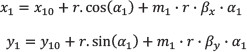
Because the turn manoeuvres are not parameterized by time but by an angle shift, trochoidal curve equations (1) and (2) can be rewritten as follows:


where

α ∈ 〈startAngle, start Angle + angle〉, angle ∈; 〈−2π, 2π〉.
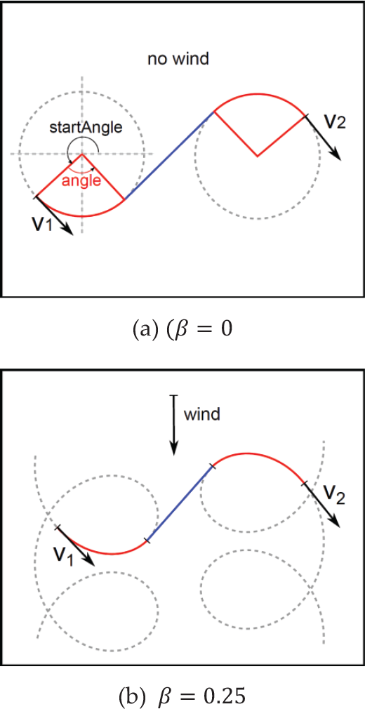
The startAngle parameter determines the initial position in the trochoid (this corresponds to an angle in a circle, see Figure 5) where the curve is tangent to the state's airspeed direction vector. The angle parameter corresponds to the manoeuvre's position shift along the trochoid measured from a given state's position (see Figure 5). Parameter r is an aircraft's turn radius and V W_X and V W_Y are corresponding components of the wind vector. x0 and y0 specify the position of the trochoid in space. The angleXY is the aircraft's heading used to estimate the startAngle according to the following equation:

for left and right turns respectively.
We know the wind vector that we consider constant during the whole planning process. From the known track's heading (ground speed direction vector), which needs to be continuous and the known aircraft's airspeed (direction and aircraft's heading is unknown) we can estimate angleXY according to Figure 3 and the following equations. We substitute angleXY to Equation (5) and then to Equations (3) and (4) to correctly place the trochoids (see Figure 4).

Estimation of angleXY parameter with given ground speed direction, airspeed magnitude and known wind vector.

Modification of flight manoeuvres for different start configurations.
Modification of Dubins car problem.
Obviously:

where Vg is ground speed. Then we can obtain the ground speed magnitude as:

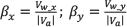
By projecting the wind vector to the ground speed vector we get:

and from the right-angled triangles we get:

By substituting (8) and (9) to (7) we estimate the ground speed magnitude and calculate the required airspeed direction (angleXY) as:

4.2.2 New straight flight manoeuvre
The effect of applying the straight flight manoeuvre in wind is straightforward and can be expressed by Equation (6). New straight flight and turn manoeuvres are shown in Figure 4 for different values of an aircraft's heading.
4.2.3 Connecting two states
When planning a path between two state configurations without obstacles, we use a modification of Dubins curves where the turn elements are trochoidal curves connected with a straight element (see Figure 5(b)). This connection of three manoeuvres is called a Smooth manoeuvre and is used for the estimation of heuristics and for smoothing the planned trajectory.
The initial trochoid is placed so that it passes through the initial state and is tangent to its direction vector. The startAngle is estimated accordingly. The second trochoid is placed similarly with respect to the second state.
Next, we need to find a tangent to both trochoids representing the straight manoeuvre between the turns. If there are more solutions to these manoeuvres we select the shortest one. The mechanism of finding the tangents differs according to the turn sides in the three consecutive manoeuvres. We distinguish two cases: i) turn – straight segment - same side turn and ii) turn - straight segment - opposite side turn (see Figure 6).

Connection of manoeuvres. L/R means left/right side turns and S represents straight flight element.
To describe the trochoids, we use constants
Then for points (x1, y1) of the first trochoid and (x2, y2) of the second trochoid holds:
and:

where α1, α2 ∈ 〈start Angle, start Angle + angle〉, angle ∈ 〈−2π, 2π〉, m1, m2 = sign(angle)
4.2.3.1 Same side turn
As can be seen in Figure 6(a) in this case the trochoids are only translated one to the other where the direction of the straight segments connecting these two curves is parallel to a translation vector t = [tx ty]. Because a trochoid is a periodic function, there are an infinite number of translations vectors. The directions on the ends of straight segments are the same (m1 = m2), so we can determine the translation vectors by the substitution a1 = a2 + n · 2π.
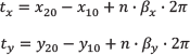
Then we need to find the value of angle α, which specifies the first turn length, so that one of the translation vectors is tangential to a point on the first curve given by α. From that point we can apply a particular translation and find the straight manoeuvre that tangentially connects the two trochoids. This method is described in detail in [16].
4.2.3.2 Opposite side turn
In this case the trochoids are centrally symmetric according to a point S = [Sx Sy] and again there are an infinite number of these points (see Figure 6(b)). The directions on the ends of the straight segment are the same, but either the first or the second turn radius is negative (m1 = –m2). We can determine the centres of symmetry by the substitution α1 = 0, α2 = (2n + 1)π.

where n ∈ ℤ.
Straight manoeuvres need to pass through one of these points. Then we need to find the value of parameter α so that the following straight element passes one of the centres of symmetry.
4.2.4 Modifications of heuristic function
As described in Section 3, the AA* algorithm uses Dubins curves to estimate the heuristics from a given state to the goal. However, McGee et al. [10] proved that for certain configurations in the presence of wind, non-Dubins manoeuvres need to be applied for time-optimal planning.
To be able to use the manoeuvres presented above and not to reduce the optimality of the algorithm, we defined a so-called irregular zone around a current state. If the target state lies outside the zone, we can be sure that our manoeuvres are time-optimal. For states inside this zone we are not sure whether they can be reached by Dubins manoeuvres and thus we use other less informative heuristics, such as the Cartesian distance. Another effect of this approach is that outside the irregular zone, only the curve-straight-curve elements can be time-optimal and thus we do not need to consider the curve-curve-curve Dubins elements. The size of the irregular zone and its description requires complex derivation, which is given in Appendix A.1.
5. Experiments
To verify the proposed methods, we deployed the modified AA* algorithm on a real fixed wing UAV (see Figure 7). We compared plan execution precision in cases with plans found by a regular AA* algorithm and with plans found by the AA* modified for planning in wind. Tests were conducted in a the presence of approximately 5m/s wind in different directions (measured by Kestrel autopilot on the basis of airspeed and GPS comparison) and the UAV's airspeed was 15m/s, giving β = 0.33. The scenario consisted of three waypoints placed in a triangle (see Figures 9 to 12). The blue line in Figures 9–12 represents the planned trajectory that starts at the first waypoint (WP1) then proceeds via WP2 and WP3 and ends again in WP1. The green line shows the real recorded trajectory of the UAV and black arrows emphasize different turn radii in individual cases. Red crosses are plan samples uploaded to the UAV's autopilot. The sampling period is proportional to the planned flight time in straight segments and the turning rate in turn manoeuvres.

Procerus UAV with Kestrel autopilot.

Probability distribution of track following error.
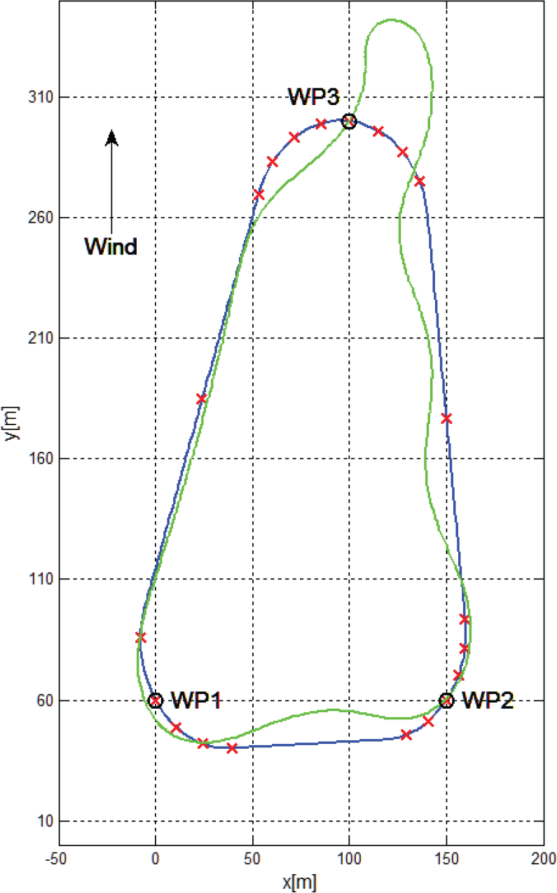
Planning with Dubins curves in south wind.

Planning with trochoidal curves in south wind.

Planning with Dubins curves in east wind.
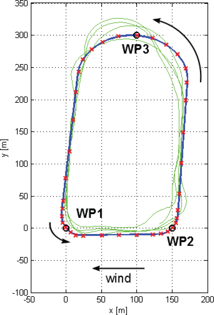
Planning with trochoidal curves in east wind.
The largest deviations from the plan occurred near the third waypoint where the UAV turns to the direction of the wind. The speed of the wind and the aircraft add together and thus, a much larger turn radius is needed. This makes the trajectories created with Dubins curves with a constant turn radius hard to follow. Trajectories created with trochoidal curves, adapted to the wind speed and direction, are followed much more precisely. On the other hand, when the radius of the scheduled turns is larger than necessary, the trajectory gets shifted inwards of the turns (noticeable in Figure 11). This behaviour is caused by a navigational feature of the autopilot that switches the current waypoint target to the next one whenever the UAV reaches a predefined boundary around the waypoint (in our case 50m). This feature makes waypoint passing easier but causes the UAV's track to be shifted inwards of the turns. A modified planner can partially deal with this problem as well, because it schedules sharper curves whenever possible. Other errors are caused mainly by dynamic changes of wind during the flight. The reason why we show only one flight over the same area in Figures 9 and 10 is that wind conditions during the experiment were not stable for a longer period of time. Figure 8 shows the probability that the track following error is greater than the given distance in both East wind situations.
6. Conclusion and Future Work
In this paper we presented a novel approach for trajectory planning for Unmanned Aerial Vehicles (UAVs) in the presence of wind, based on a modified Accelerated A* algorithm. In contrast to any-time methods, the AA* approach optimally plans the whole UAV's trajectory. This modified algorithm was deployed and tested on a real UAV at a wind speed of 5m/s and achieved significantly better results than the original AA* in terms of the precision of plan execution.
In future research we would like to give evidence that in contrast to any-time methods, the AA* approach is more suitable for purposes of distributed cooperative trajectory conflict resolution, as stated in [12]. Furthermore, we would like to address the following topics: (i) modelling the uncertainty of plan execution for safer collision avoidance and (ii) modelling wind changes in different locations and altitudes. Currently, we are working on temporal planning in wind on more sophisticated missions.
7. Acknowledgements
The research described in this paper was supported by the Czech Ministry of Defence grant OVCVUT2010001, the U.S. Army grant W911NF-11-1-0252 and the Grant Agency of the Czech Technical University in Prague grant SGS13/078/OHK3/1T/13.