
Abstract
The transformation of the mean and variance of a normally distributed random variable was considered through three different nonlinear functions: sin(x), cos(x), and xk, where k is a positive integer. The true mean and variance of the random variable after these transformations is theoretically derived within, and verified with respect to Monte Carlo experiments. These statistics are used as a reference in order to compare the accuracy of two different linearization techniques: analytical linearization used in the Extended Kalman Filter (EKF) and statistical linearization used in the Unscented Kalman Filter (UKF). This comparison demonstrated the advantage of using the unscented transformation in estimating the mean after transforming through each of the considered nonlinear functions. However, the variance estimation led to mixed results in terms of which linearization technique provided the best performance. As an additional analysis, the unscented transformation was evaluated with respect to its primary scaling parameter. A nonlinear filtering example is presented to demonstrate the usefulness of the theoretically derived results.
1. Introduction
It is necessary in state [1] and parameter [2,3] estimation problems to estimate the mean and covariance of a random signal after propagating through a nonlinear function. The Extended Kalman Filter (EKF) [4] and Unscented Kalman Filter (UKF) [5] are two different estimators commonly used for nonlinear state estimation purposes. The EKF uses an analytical linearization for dealing with the nonlinearity in the transformation, while the UKF features a statistical linearization approach called the “unscented transformation” [5]. Both filters have been used for various sensor fusion applications, such as Global Positioning System/Inertial Navigation System (GPS/INS) integration [6–10], bearing-only tracking [11,12], and relative navigation [13]. The EKF and UKF have also been used for robotics applications including inertial and vision sensor fusion [14–16], tracking of people using mobile robots [17,18], surgical robots [19], indoor attitude and heading estimation [20], robot localization [21–23], and Simultaneous Localization and Mapping (SLAM) [24–27].
The differences in the performance of the EKF and UKF have been compared in various efforts; however, these comparisons were either empirical or based on simulation studies, and do not offer analytical insight into the linearization process. Additionally, the comparison of these two filters has led to inconsistent conclusions among different research groups. Some researchers have reported for GPS/INS sensor fusion [10], spacecraft attitude estimation [28], bearing-only tracking [11,12], radar tracking [29], and simulation studies of the Van der Pol oscillator, induction machine, reversible reaction, and gas turbine hybrid systems [30] that the UKF performs consistently and significantly better than the EKF. However, other researchers found that the UKF only outperformed the EKF for GPS/INS sensor fusion under large initialization errors [9,31–33]. Slight performance advantage of the UKF over the EKF was reported for angles-based navigation [34], GPS/INS position estimation [35], state estimation of induction motors [36], and aerodynamic parameter estimation [37]. Some studies of the problems of aircraft attitude estimation [6,8], ballistic missile tracking [38] and quaternion motion for human tracking [39] found insignificant differences in EKF and UKF performance. Due to the inconsistencies in the reported EKF and UKF performance, a detailed evaluation method was considered necessary. Every data point that can be provided becomes important in shaping the overall impressions on these two filters. Since most existing comparison and analysis for nonlinear filters is experimentally based, some theoretical analysis is beneficial to the research field.
The main contribution of this paper is a detailed comparison of the analytical linearization technique of the EKF with the unscented transformation of the UKF with respect to three different nonlinear functions, using analytically determined values of the true statistics after the transformation. The analytical derivations provide a computationally efficient truth reference for the nonlinear transformation of statistics. Specifically, the considered functions are sin(x), cos(x), and x k , where k is a positive integer. These functions were selected to capture nonlinearities that are commonly encountered in different estimation problems. Additionally, these functions contain desirable analytical properties which allow for the derivation of the true mean and variance after the transformation. The polynomial function is particularly useful because its analytical properties can be used to derive properties of other nonlinear functions through their Taylor series approximations. This process is demonstrated for the trigonometric functions, which were presented because their statistics can be represented with a closed-form solution. Also, the analytically derived results, as well as the method used to obtain them, could be useful for other analytical research in different applications.
To facilitate the analytical derivations, the distribution of the random signal is assumed to be Gaussian, with known mean and standard deviation. This distribution was selected because the propagation of Gaussian noise through nonlinear equations is a commonly considered problem in the technical community [6–13], and is the distribution that is assumed by both the EKF and UKF. Other nonlinear estimators such as particle filters can be used to approximate other distributions if necessary [1,7,40,41].
This rest of the paper is organized as follows. First, the true mean and variance after the transformation of a zero mean normally distributed variable are considered in Section 2. In Section 3, these relationships are extended in order to determine the true statistics after the transformation of a non-zero mean random variable. In Section 4, the comparison of the analytical and statistical linearization techniques is presented. A nonlinear filtering example is provided in Section 5, followed by the conclusions in Section 6.
2. Nonlinear Transformations of a Zero Mean Normally Distributed Variable
Consider a normally distributed random variable, x, with zero mean, and variance, σ2, i.e.,


Let y be some nonlinear function of x, y = g(x). For each of these nonlinear functions, the mean and variance after the nonlinear transformation can be determined using the expectation operator [42]:

2.1. Polynomial Functions of Zero Mean Variables
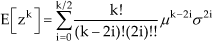
The nonlinear function y = x k is considered as a general case to capture the effects of polynomials, where k is a positive integer. For this function, the expectation integral does not need to be evaluated; instead, the moment generating function, M(t), can be used to derive the moments of this function [42]:

Thus, the mean of y is given by:

where !! is the double factorial operator [43]. To calculate the variance of y, the computational formula of the variance is used [42]:

Using (5) and (6), the variance of y = x k is calculated using:

2.2. Trigonometric Functions of Zero Mean Variables
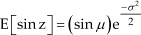
Consider the nonlinear function y = sin(x). Solving (3) directly for this function is not a trivial matter. However, if the sine function is expanded using its Taylor series, the expectation becomes:
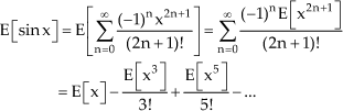
By applying (5), the expectation in (8) gives
For y = cos(x), a similar procedure is used to calculate the mean of y:
Applying (5) leads to the following simplifications:

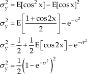
Next, the variances for the sine and cosine functions are calculated using (6). The variance of the sine function is given by:

The variance of the cosine function is given by:
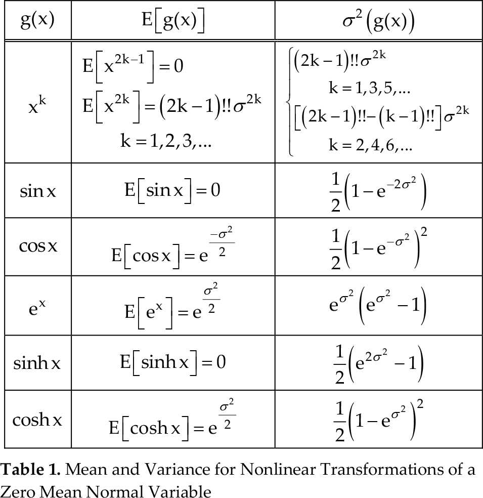
This method of using the statistical properties of the polynomial function from (5) and utilizing the Taylor series expansion can be applied to other nonlinear functions. The details are omitted here for conciseness, but this method was applied to some additional nonlinear functions to demonstrate its usefulness. The results from this analysis are summarized in Table 1.
Mean and Variance for Nonlinear Transformations of a Zero Mean Normal Variable
3. Nonlinear Transformations of a Non-Zero Mean Normally Distributed Variablet1
Consider a normally distributed random variable, z, with mean, μ, and variance, σ2, i.e.,
3.1. Polynomial Functions of Non-Zero Mean Variables
First the nonlinear function y = z k is considered. The expected value of y can be obtained using the binomial expansion [42]:

where the expectations of x are given by (5):
The variance is then determined using (6) and (14) to be:

3.2. Trigonometric Functions of Non-Zero Mean Variables
Next the nonlinear function y = sin(z) is considered. The expected value of y can be obtained by taking advantage of the relationship of z to x, as well as trigonometric identities:

Using the previously determined expectations of the sine and cosine functions with respect to x in Table 1, the expected value of y is determined as:
The variance is then derived from (6) and (17), as well as Table 1:

For the nonlinear function y = cos(z), similar procedures can be used as for the sine function, and the expected value and variance after the transformation has been found as:


The results of this analysis are summarized in Table 2.
Mean and Variance for Nonlinear Transformations of a Non-Zero Mean Normal Variable

4. Comparison of Linearization Techniques in Nonlinear Filters
Consider a nonlinear transformation of the form y = g(z), where


These values were calculated using (21) and (22) for each of the three considered nonlinear transformations and the results are summarized in Table 3.
Mean and Variance Estimates from Analytical Linearization

The Unscented Transformation (UT) is a statistical linearization technique used by the UKF. For the considered scalar case, the UT consists of the calculation of three sigma points:

where α is the primary sigma point scaling parameter, which is suggested to vary between 0.001 and 1 [10]. Weighted averages are taken to recover the mean and variance of these sigma points, as in:
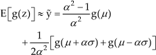
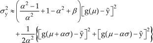
where
Since the linearization process is a function of the prior mean and variance, plots were generated to illustrate the differences between the analytical and statistical linearization techniques. Additionally, the Monte Carlo method was included to verify the theoretically derived results, i.e., n = 105 points were generated from the prior distribution, propagated through the nonlinear function, and then the mean and variance statistics were calculated, as in

The differences between the Monte Carlo and theoretical estimates for the mean and variance are negligible for all of the considered cases, thus demonstrating the validity of the theoretically derived equations. For the unscented transformation, four different cases of α were considered: 0.25, 0.5, 0.75, and 1.0. These values were selected to represent a few cases in the range of possible values for α. Each presented figure shows the error in the transformed mean or variance estimate from the linearization process as compared to the theoretically derived truth from Table 2. These errors are plotted with respect to the prior standard deviation, σ.
First, two cases of the nonlinear function y = z k are considered: k = 2 and k = 3. For both cases, E[z] = 0.1. Alternatively, due to the relationship between z and x, this function can be considered as y = (x+0.1) k . For k = 2, the mean and variance estimates for each case of α were the same, and therefore only one line is plotted for the UT, as shown in Figure 1.
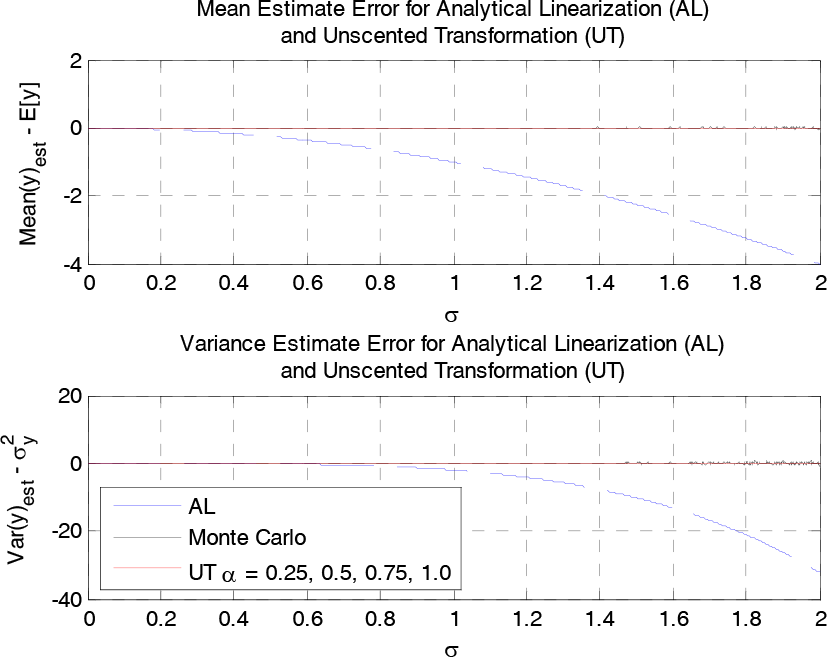
Mean and Variance Estimate Errors for y = (x + 0.1)2
It is shown in Figure 1 that the AL error increases as the prior variance increases, while the UT provides perfect estimation of both the mean and the variance. As expected, the Monte Carlo method provides near perfect estimation of the statistics. For k = 3, the mean estimate again is not a function of α; however, the variance estimate is function of α. The results for this case are shown in Figure 2.
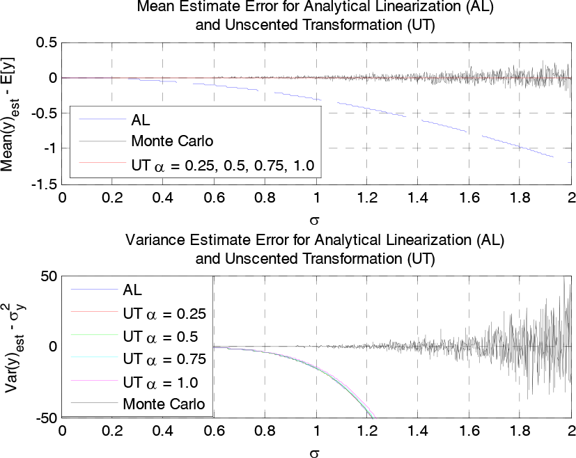
Mean and Variance Estimate Errors for y = (x + 0.1)3
For the case shown in Figure 2, the AL again shows an increasing error trend with prior variance. The UT provides perfect mean estimation, but the variance estimate is now only slightly more accurate than the AL, with α = 1.0 giving the greatest accuracy. For this case, errors in the Monte Carlo method become more apparent as the prior variance increases. This indicates that a larger number of points would be required to accurately estimate the statistics. This particular case demonstrates the usefulness of the theoretically derived statistics in Table 2, as the Monte Carlo method can become inaccurate even for a reasonably large number of points. Therefore, using Monte Carlo as a truth reference may be invalid under certain conditions. The derived statistics in Table 2 are clearly advantageous for this case in terms of computation and accuracy.
The next considered case is y = sin(x). The mean estimate for this case is identically zero for both techniques, so it is not shown. The variance estimate, however, shown in Figure 3, shows that the UT contains greater accuracy than the AL for all cases of α, with α = 1.0 giving the best variance estimate.

Variance Estimate Error for y = sin(x)
Next, two non-zero mean cases are considered for the sine function. The mean and variance estimates for y = sin(z) with E[z] = π/4 are shown in Figure 4, and similarly for y = sin(z) with E[z] = π/2 in Figure 5.
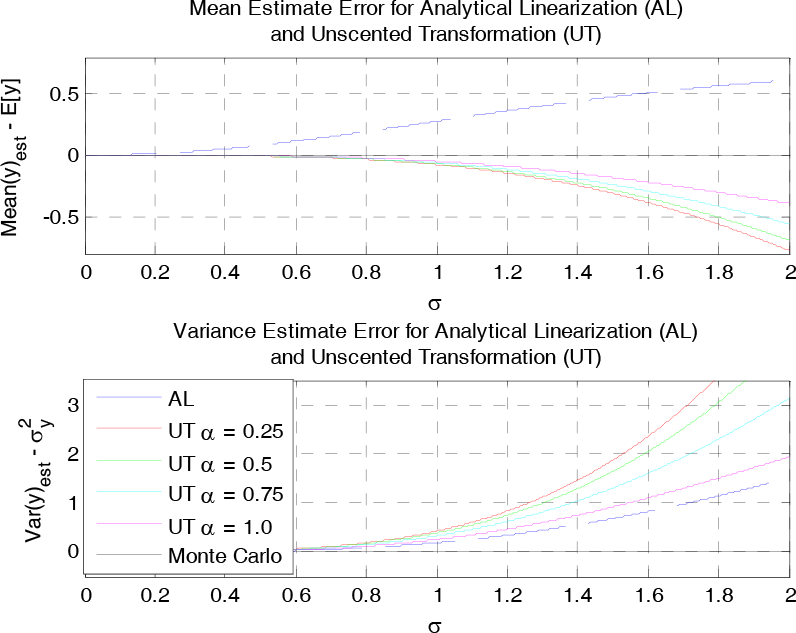
Mean and Variance Estimate Errors for y = sin(x+π/4)

Mean and Variance Estimate Errors for y = sin(x+π/2)
For the cases shown in Figure 4 and Figure 5, the UT provides more accurate mean estimation; however, the AL provides a more accurate variance estimate. Comparable cases for the cosine function were generated, and yielded equivalent results to those of the sine function, as expected, following the co-function identities, i.e., cos(x) = sin(π/2–x). For each of the cases for the sine and cosine functions, it is interesting to note that the value of α = 1.0 gave the most accurate mean and variance estimates for the UT. Also, the Monte Carlo method provides near perfect estimation of the statistics, as expected.
Figure 4 and Figure 5 show specific cases of the prior mean in order to give snapshots of the performance. To more fully capture the effects of different means, the AL and UT were evaluated for the sine function over a set of values for the standard deviation ranging from 0 to 2 and for the mean ranging from 0 to π/2. Only the case of α = 1.0 was considered here for the UT. The absolute value of the mean estimate error and variance estimate error are displayed for AL in Figure 6 and UT in Figure 7 as contours. In these figures, the darker areas indicate higher linearization errors with respect to the analytical truth.
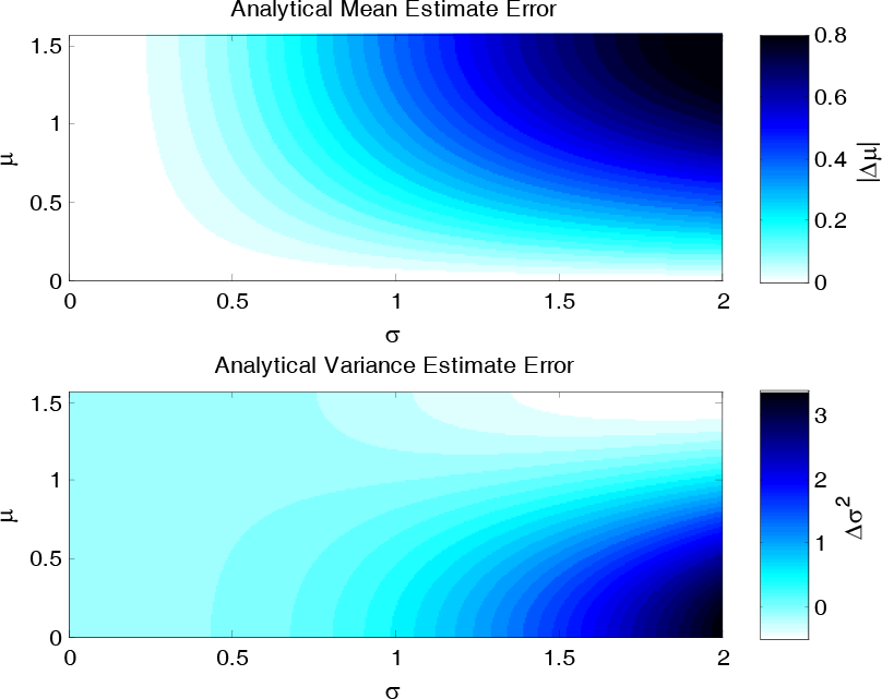
Analytical Linearization Error for y = sin(z)

Unscented Transformation Error for y = sin(z)
There are two important observations to make in Figure 6 and Figure 7. First, for all cases of prior mean and standard deviation, the UT yields more accurate estimation of the mean. Second, the variance estimate errors of the AL are sometimes better than the UT, and vice versa. This is demonstrated by the different shapes of the contour graphs, with AL having higher errors for smaller means and the UT having higher errors for larger means. Because of this observation, neither the AL nor UT can claim better estimation of the variance for all cases.
5. Nonlinear Filtering Example
In order to demonstrate the usefulness of the derived analytical relationships, an example of a nonlinear filtering problem is considered. Consider the following discrete-time nonlinear system:

where k is the discrete time index, x is the state, y is the output, and v is the measurement noise with known variance, R. This problem is approached with the EKF, the UKF, a theoretical filter which uses the relationships summarized in Table 2, a Monte Carlo based filter, and a particle filter. For this implementation of the UKF, the scaling parameters were set to α = 1.0 and β = 2. The Monte Carlo filter generated n = 106 points at each time step from the prior distribution to recover the statistics after the nonlinear transformation using (26). Note that this Monte Carlo filter is not a particle filter, but is instead a Kalman filter that uses the Monte Carlo method to determine the a priori statistics at each time step. This Monte Carlo filter is a statistical means of approximating the theoretical filter. A linear Kalman filter measurement update [1] is used for the EKF, UKF, theoretical, and Monte Carlo filters, since the output equation is linear. To provide additional comparison, a simple Sampling Importance Resampling (SIR) particle filter [40] was implemented using 106 particles.
First, the true state trajectory is determined for an initial state,
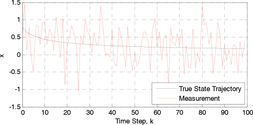
Nonlinear Filtering Example: State and Measurement
Using this measurement, each filter algorithm is executed for 100 discrete time steps, each using assumed initial conditions:

where P is the variance of the state. These initial conditions were selected to capture the effects of a reasonably large initialization error. Note that the initial error was selected as one standard deviation from the assumed initial variance. The state estimation error results of this simulation are shown in Figure 9.

Nonlinear Filtering Example: Estimation Error
Negligible differences are shown in Figure 9 between the Monte Carlo and theoretical filters. To quantify the performance of each filter, the root mean square error (RMSE) was calculated, and is shown in Table 4.
Nonlinear Filtering Example: Root Mean Square Error

From these results, a slight performance advantage is demonstrated for the UKF over the EKF, and a more significant performance advantage is shown for the Monte Carlo and theoretical filters over both the EKF and the UKF. This improvement comes purely from the removal of the linearization errors that are incurred by the EKF and UKF. The particle filter was able to achieve the highest accuracy, due to the removal of the Gaussian noise assumption that is required by the other methods. This indicates that even with perfect linearization, Kalman-based filtering techniques may not be as effective as particle filtering.
6. Conclusions
The results of a comparison of analytical linearization and unscented transformation techniques to recover the mean and variance after three different nonlinear transformations were presented in this paper. The true statistics were theoretically derived for each of the considered functions in order to compare the errors of the different methods. These theoretical results were verified with respect to Monte Carlo simulations. For all of the considered cases, the unscented transformation yielded equal or greater accuracy in the estimation of the mean. However, mixed conclusions were reached about the accuracy of the variance. For some cases the analytical linearization obtained greater accuracy than the unscented transformation, while for other cases the opposite was noticed. Another interesting observation is that for each function, increasing α in the unscented transformation gave equal or better accuracy. Additionally, a nonlinear filtering example was given to demonstrate the effectiveness of the theoretical estimates in practice, either as a validation tool or for implementation. This example showed that there is room for improvement in both the EKF and the UKF in terms of linearization errors for certain applications, and that a particle filter is still able to outperform a Kalman-based filter even with no linearization error.
Footnotes
7. Acknowledgments
This research was partially supported by NASA grant # NNX10AI14G.