Sage Journals: Discover world-class research

Abstract

In recent years, the use of imaging sensors that produce a three-dimensional representation of the environment has become an efficient solution to increase the degree of perception of autonomous mobile robots. Accurate and dense 3D point clouds can be generated from traditional stereo systems and laser scanners or from the new generation of RGB-D cameras, representing a versatile, reliable and cost-effective solution that is rapidly gaining interest within the robotics community. For autonomous mobile robots, it is critical to assess the traversability of the surrounding environment, especially when driving across natural terrain. In this paper, a novel approach to detect traversable and non-traversable regions of the environment from a depth image is presented that could enhance mobility and safety through integration with localization, control and planning methods.

The proposed algorithm is based on the analysis of the normal vector of a surface obtained through Principal Component Analysis and it leads to the definition of a novel, so defined, Unevenness Point Descriptor. Experimental results, obtained with vehicles operating in indoor and outdoor environments, are presented to validate this approach.

Keywords

Rough-Terrain Mobile Robots 3D Perception Terrain Traversability Unevenness Point Descriptor

1. Introduction

Future autonomous mobile robots will take part in our daily lives and they will interact with much of our environment. In order to accomplish its task, it is critical for a robot to be endowed with advanced perception capabilities. In this regard, depth perception, i.e., the visual ability to perceive the world in three dimensions and the distance of an object, is gaining new interest in the robotics community thanks to the introduction of the next generation of RGB-D cameras, including Microsoft Kinect [1] and ASUS Xtion [2]. They provide information on the distance between the sensor and a point in the space, eventually adding information about the colour. By collecting sets of distances, it is possible to create a 3D map of the environment that can be converted into the vehicle's reference frame, obtaining what is usually referred to as a “point cloud”. RGB-D cameras feature remarkable accuracy, cost effectiveness, compactness, low power consumption and they are lightweight and well suited for robotics applications. However, perception based on depth cameras cannot be implemented without an efficient algorithmic approach that is able to read and interpret raw data.

The problem of image interpretation has been widely studied [3], [4], [5], [6], [7]. From a mathematical point of view, describing a specific characteristic of an object in order to give a perceptive meaning is not easy. This issue is called “semantic perception” [8].

In this work, a novel approach for terrain roughness estimation is proposed based on the use of normal vectors. Non-traversable obstacles or highly irregular terrain can be detected by an autonomous vehicle along its path toward a target both in indoor and outdoor scenarios. Research in this field generally refers to two indices: the roughness and the inclination index [9], [10]. The former is defined as the variance of the elevation values in a specific region of the environment, whereas the latter can be obtained as the average angle of adjacent elevation values with respect to their neighbours [11]. The independent application of these often leads to poor results or misclassifications. For example, the roughness index will flag as uneven a low-steep slope with regular surface, due to the increasing value in elevation. Conversely, the inclination angle will fail to correctly recognize irregular terrain, whose local inclinations appear null or result in a low average inclination.

Here, a novel point descriptor, a so-called Unevenness Point Descriptor (UPD), is introduced that takes into account both the inclination and roughness of the local surface. Hence, rather than using two scalar indices, the UPD represents a simple and robust choice that gives a better description of the traversability properties of the surrounding terrain.

For the extensive testing of the system during its development, two robotic platforms were used: the all-terrain rover Dune and an experimental agricultural tractor. Dune, built at the Applied Mechanics Laboratory of the University of Salento, is shown in Fig. 1. The robot was equipped with a Microsoft Kinect RGB-D camera during indoor experiments. The Point Grey XB3 stereo system was used, instead, with the test bed tractor to generate 3D point clouds in outdoor environments.

Figure 1.

The all-terrain rover Dune equipped with the Microsoft Kinect camera.

The paper is organized as follows. In Section 2, an overview of the system is presented along with the description of the algorithm to generate a 3D representation of the environment. In Section 3, basic concepts of point feature and surface representation are recalled. The proposed UPD is introduced in Section 4 along with its application to terrain analysis. Next, Section 5 validates the proposed approach in indoor and outdoor experiments. Relevant results are shown in Section 6.

2. System overview

The rover Dune is an independently controlled four-wheel-drive/four-wheel-steer mobile robot, also featuring a rocker-type suspension system, which provides remarkable mobility on natural terrain, allowing the rover to safely traverse rocks over one and half times its wheel diameter [12]. The robot is equipped with wheel and steer encoders and an IMU to measure robot orientation. Its operational speed ranges from 2 to 30cm/s.

A Microsoft Kinect sensor was also mounted on the front of the vehicle, as shown in Fig. 1. The depth camera provides a 640×480 RGB-D image at 30Hz, corresponding to a field of view approximately 5m long and 4m wide on the ground plane. It comprises a RGB camera and 3D depth sensor. The RGB camera provides eight-bit images with a resolution of 640×480 pixels. The 3D depth sensor consists of an infrared laser emitter and a monochrome depth camera that provides “light coding” to estimate the distance of each pixel in the image. In more detail, the laser emitter projects pseudo-random patterns of speckles on the environment and the monochrome camera is able to read the infrared pattern. By combining the information of the RGB and monochrome camera, it is possible to obtain a 3D reconstruction of the scene. However, the Kinect sensor is not able to acquire data in outdoor environments due to the limitations of the brightness intensity range. For this reason, an outdoor 3D reconstruction was performed using the multi-baseline, IEEE-1394b (800Mb/s) stereo camera, Point Grey Bumblebee XB3 [13]. It also features 1.3 mega-pixel sensors and has two baselines (12/24cm) available for stereo processing, corresponding to a field of view approximately 24m long and 18m wide on the ground plane. The extended baseline and high resolution provide more precision at longer ranges, while the narrow baseline improves close range matching and minimum-range limitations [14].

Processing of the sensor raw data was performed using the Point Cloud Library (PCL) [15]. PCL presents an advanced and extensive approach to the subject of 3D perception, providing support for all the common 3D building blocks that the applications require. The library contains state-of-the-art algorithms for filtering, feature estimation, surface reconstruction, registration, model fitting and segmentation.

In Fig. 2, the overall process pipeline of the system is shown. First, the original image is acquired and the 3D point cloud can be generated. Each point p_i has six coordinates: p_i (x, y, z, r, g, b), where the first three components are the Cartesian coordinates (x, y, z) and the last three coordinates are the RGB colour information. In order to mitigate the problems connected with measurement noise, a pre-processing phase is applied. This includes a cut-off filter, a statistical outlier removal filter and a downsampling filter.

Figure 2.

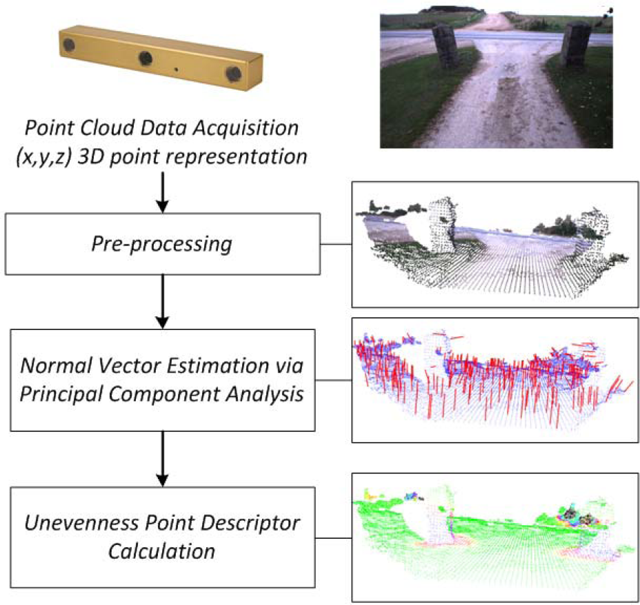
The process pipeline of the proposed system.

The cut-off filter eliminates points in the out-of-range region. The outlier removal module filters the points located close to an object but that do not actually belong to it. The downsampling process reduces the number of points per volume unit by statistical analysis. More specifically, a point cloud is generally composed of “dense” and “not dense” areas. A volume unit is referred to as dense if it is rich in information; otherwise, it is referred to as not dense. The downsampling process checks every volume unit or voxel of the image and, where the cloud is dense, it computes the average pixel in order to gain a good approximation of the information of the voxel. This reduces the redundancy of the information in the point cloud with computational advantages during post-processing. In summary, the pre-processing stage produces two different advantages: the image becomes clearer and the computational burden of post-processing is reduced.

3. Point feature representation

In the context of semantic perception, the concept of a “local descriptor” was introduced to describe the property of a region of the space in a single point [16], [17]. Using a local descriptor, it is possible to define and represent several characteristics of this point according to the specific application. For example, in [18] the authors discriminate shapes and planes by using point feature representation and their geometric primitives.

In order to give a mathematical formulation to the concept of a local descriptor, let us consider image I as a set of points in Cartesian coordinates I = {p ∈ ℛ³} and let us define point p_q as a query point (point where the descriptor is calculated). Hence, the concept of neighbourhood is defined as the set of points:

P^{k} = \{p_{i}^{k} \in R^{3} : ‖p_{i}^{k} - p_{q}‖ \leq d_{m}\}

(1)

where d_m, defined as the search radius, is the maximum distance between p_q and each neighbour, k is the number of neighbours of p_q and ‖·‖ is a generic norm (without a loss of generality we refer to the Euclidean distance). The k-points in the neighbouring vicinity of p_q will be called “neighbours”. Therefore, a point feature representation can be indicated as the vector function F that describes the information content of P^k and set of neighbours of p_q, according to a specific feature:

F ({p_{q}, P}^{k}) = \{x_{1}^{q}, x_{2}^{q}, \dots, x_{n}^{q}\}

(2)

where $x_{i}^{q}, i \in \{1, 2, \dots, n\}$ , i ∈ {1, 2, …,n} is the i-th dimension of the descriptor calculated in the query point p_q. Let Γ be the measure of similarity that describes the difference between two different points p₁ and p₂, with their associated descriptors F₁ and F₂, and d be their distance:

Γ = d (F_{1}, F_{2})

(3)

Then d can be considered as the degree of similarity between the given points. If d → 0 the points described by F₁ and F₂ can be considered similar according to the specific descriptor. If d increases the points are less similar, i.e., they will feature different geometric characteristics. By including a large number of neighbours, the descriptor will have more information about its surrounding neighbourhood.

In general, the confidence of the descriptor is represented by the ability to differentiate points in the presence of rigid transformations, noise, sampling variations and changes in scale or illumination [18].

3.1 Normal estimation by Principal Component Analysis

The set of neighbours P^k, at a query point p_q, can be used to assess the surface geometry in the vicinity of p_q. For example, a typical problem is to determine the orientation of a given surface in a specific coordinate frame; this can be done through the estimation of its normal vector. In order to estimate the normal vector, Principal Component Analysis (PCA) can be applied. Although many different normal estimation methods exist, the simplest method is based on the first order 3D plane fitting, as proposed in [20].

This problem can be seen as the problem of determining the normal vector of the tangent plane to the surface in the query point [8], [18]. The tangent plane can be obtained as the fitting with the least square in P^k. A plane can be represented as an application point x and its normal vector $\vec{n}$ , with the distance of each point p_i ∈ P^k from the plane defined as $l_{i} = (p_{i} - x) ∙ \vec{n}$ . If we consider:

x = \bar{p} = \frac{1}{k} \cdot \sum_{i = 1}^{k} p_{i}

(4)

as the centroid of P^k, the solution for $\vec{n}$ can be obtained by analysing the Eigenvalues and Eigenvectors of the covariance matrix C ∈ ℛ^3×3 of P^k, expressed by:

\begin{matrix} C = \frac{1}{k} \sum_{i = 1}^{k} ξ_{i} \cdot (p_{i} - \bar{p}) \cdot {(p_{i} - \bar{p})}^{T} \\ C \cdot \vec{v_{j}} = λ_{j} \cdot \vec{v_{j}}, j \in \{0,1, 2\} \end{matrix}

(5)

The term ξ_i is the possible weight for p_i and it is usually considered as unitary. The covariance matrix C is symmetric, positive-definite, and its Eigenvalues are real. The Eigenvectors $\vec{v_{j}}$ form an orthogonal subspace and are the principal components of P^k. If we suppose 0 ≤ λ₀ ≤ λ₁ ≤ λ₂ are the Eigenvalues of C, then the Eigenvector of the Eigenvalue λ₀ represents the approximation of the normal vector $\vec{n} = \{n_{x}, n_{y}, n_{z}\}$ or its opposite $- \vec{n}$ .

It should be noted that the ambiguity on the sign of the normal vector is not analytically solvable; it is generally estimated through the analysis of the other Eigenvectors that complete the Eigenspace. This means that every surface will have two sets of normal vectors. Here, we will conventionally consider only the normal vector pointing upward. It may not point directly up, but it will have an upward component to it.

4. Terrain analysis via normal vectors

Let us consider the query point p_q, and its neighbouring vicinity P^k, computed as defined in Section 3. Given the $P^{k}$ normal vectors with i=1, 2, …, k, where k is the number of neighbours, it is possible to compute the vector sum of the normal vectors

{\vec{r}}_{k}^{q} = {\vec{n}}_{1} + {\vec{n}}_{2} + \dots {\vec{n}}_{k} = \sum_{i = 1}^{k} {\vec{n}}_{i}

(6)

Then the Unevenness Point Descriptor (UPD) in p_q, can be defined as:

U P D = F ({p_{q}, P}^{k}) = \{r_{x}^{q}, r_{y}^{q}, r_{z}^{q}, ζ_{k}^{q}\}

(7)

where $r_{x}^{q}, r_{y}^{q}, r_{z}^{q}$ are the components of the vector ${\vec{r}}_{k}^{q}$ and $ζ_{k}^{q}$ is given by:

ζ_{k}^{q} = \frac{‖{\vec{r}}_{k}^{q}‖}{k}

(8)

$ζ_{k}^{q}$ can be interpreted as a local inverse “unevenness index” providing information about terrain roughness point by point. The higher the value (note that the possible maximum value is one), the more regular the neighbourhood of p_q. The unevenness index depends on the distribution of the directions of the normal vectors in the neighbourhood. A discussion about its calculation may be useful to better understand the proposed descriptor. Let us consider the following directions of the normal vectors that generate special cases:

Vectors ${\vec{n}}_{i}$ parallel $ζ_{k}^{q}$ =1 = max

Vectors ${\vec{n}}_{i}$ two by two orthogonal $ζ_{k}^{q} = \frac{\sqrt{2}}{2}$ =min

The first case has a simple solution because the sum of parallel vectors gives a vector with the same direction as all the vectors and the unitary module. One should note that the module is independent of the inclination of the surface (i.e., the presence of a slope); this gives to the unevenness point descriptor the property of invariance to the orientation of the local surface with respect to the sensor reference frame.

If the normal vectors are two by two orthogonal, the vector sum will have the (absolute) minimum norm. This case is theoretically important because it gives a physical meaning to the minima of the unevenness index. Typical cases can be encountered in the vicinity of a stair or at the intersection between floor and wall, or, more generally, in the vicinity of a strong variation in the surface inclination. Local minima of the unevenness index may also be reached in proximity of a rock or of terrain discontinuity. Let us recall that the normal vectors cannot have opposite orientation as explained in Section 3.1, where the problem of sign ambiguity has been discussed. Hence, all normal vectors should have an upward component.

In all other situations, the unevenness index $ζ_{k}^{q}$ is given by (8) and it can be used to describe locally the geometric properties of the ground.

4.1 Algorithm description

The algorithm for the estimation of the UPD can be summarized as follows:

1. Point cloud acquisition, filtering and downsampling 2. For all pi do 3. P^k selection, eq.(1) 4. Compute covariance matrix in P^k, eq. (5) 5. Compute n→_i 6. End 7. For all pi do 8. P^k selection eq.(1) 9. Compute the UPD eq.(6), (8) 10. End

Algorithm 1. Pseudocode to Estimate the Unevenness Point Descriptor

Computationally speaking, the factor that mostly affects the performance of the algorithm is the dimension of P^k. Specifically, the complexity of the algorithm increases with the dimension of P^k. Although (1) was introduced as a function of d_m, using a distance to define the neighbourhood may be problematic for field acquisitions in the presence of sparse data. In general, 3D point clouds are composed by dense and not-dense areas due to the sensor's limitations (e.g., occluded area or pixels at a large distance). In these cases, it may be more convenient to refer to the parameter k (see (6)), instead. The value of k can be fixed at the beginning of the operations selecting for every observed point the nearest k points (k-neighbours). In this way, the set P^k defined in (1) would always have the same number of points but the search radius would change according to the denseness of the point cloud. As a drawback, if the point cloud is sparse in a certain region of the space, the neighbouring vicinity may select points that belong to different surfaces, resulting in not-coherent results. This is often the case in the proximity of border regions where there is not generally enough information to fully describe the terrain. As the sensors used in this research ensure good data denseness, we will refer to d_m. In practice, its value will be fixed at the beginning of the operations based on the geometric size of the robot, as explained later in the paper.

5. Experimental results

In order to demonstrate the effectiveness of the UPD-based approach for terrain roughness evaluation, we first apply the system to simulated data. Then, the UPD is experimentally validated in real experiments performed in both indoor and outdoor scenarios.

5.1 Case study 1: simulated data

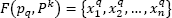
The presence of a 90 degree-corner is simulated by numerically generating two orthogonal planes whose dimensions are 1×1m with a resolution of 0.01m (the point cloud is represented by a grid with points 0.01m apart). The goal of this simulation is to evaluate the influence of the search radius d_m on the unevenness index, i.e., the fourth component of the UPD. Fig. 3 shows the results obtained applying the unevenness index using three different values of the search radius (d_m= 0.1, 0.5, 1.0 m). High values of ${\vec{n}}_{i}$ suggest regularity, low values indicate irregularity, as reflected by the colour bar associated with Fig. 3. The performance of the system is greatly affected by the search radius. If d_m is too large (d_m=1 m), all normal vectors will influence each other resulting in poor results and in difficulty in detecting the exact location of the discontinuity. Conversely, when a value d_m = 0.1m is assumed, the corner is detected with a higher resolution in a limited region of the space. As a general rule, the larger d_m, the wider the portion of the environment that is considered for the estimation of the UPD in the given query point. Therefore, all obstacles within a distance of d_m from this point will affect the index estimation. This consideration in conjunction with the knowledge of the vehicle's geometric size and the field of view of the sensor, suggests a possible approach for the optimal choice of d_m.

Figure 3.

Analysis of a 90-deg corner using the unevenness index with different values of the search radius.

In order to provide a quantitative evaluation of the system performance, in Fig. 4 a histogram analysis is shown. The histogram shows the distribution of the unevenness index using two different values of the search radius: 0.3m (red bins) and 1.0m (blue bins). In the close-up inset of Fig. 4, it is shown that a large percentage of points with high values of $ζ_{k}^{q}$ is found (see red bins in the inset) for d_m=0.3 m. The presence of points with a low value of the unevenness index signals a geometric discontinuity. One can note that, when the search radius is large (d_m=1.0m), more than 80% of components are in the range [0.75-0.85]. This demonstrates how the size of d_m can affect the value of the local minima, but not the geometric areas where the minima are found.

Figure 4.

Histogram of the unevenness index for the simulated corner shown in Fig. 3.

Finally, the UPD is compared against the existing literature for a simulated scenario featuring a ramp with a slope of 20 degrees. Fig. 5(a) shows the results obtained from the UPD-based approach. As expected, the lower border of the ramp is flagged as irregular, whereas the ramp itself is correctly labelled as traversable. In Fig. 5(b), the same scene is analysed applying the roughness index, defined in [11] as the standard deviation of the terrain elevation over a local surface that is assumed to be equal to the neighbourhood of the query point in this analysis. By relaying on terrain elevation only, the ramp is misclassified as non-traversable by the roughness index. In contrast, the UPD approach is based on the analysis of the local normal vectors providing a similar score for the ground and the ramp that are both classified as traversable.

Figure 5.

Comparison of the UPD with the roughness index for a simulated ramp. The UPD labels as traversable both ground and ramp, whereas the roughness index provides different scores B for the ground (B=B_min) and ramp (B=B_max).

5.2 Case study 2: indoor data

Experiments were performed in a laboratory environment using the rover Dune equipped with the Microsoft Kinect. The look-ahead distance of the Kinect sensor is about 4m, while the robot is 0.7m long and 0.45 m wide with a wheel diameter of 0.2m. Based on these parameters, a good choice for d_m was empirically found as d_m=0.5m, trading off between collision-free safety and good accuracy in obstacle detection. Fig. 6 shows a typical result obtained in a corridor scenario. In the upper plot of Fig. 6, the original RGB image is shown. Fig. 6(b) shows the representation of the normal vectors obtained for the same image. One should note that the normal vectors are parallel across regular surfaces such as the floor and walls, but they show different directions in the proximity of geometric discontinuities. Finally, Fig. 6(c) shows the traversability assessment of the scene based on the UPD analysis. The colour of each point is set proportionally to the value of the unevenness index.

Figure 6.

Indoor environment analysis using normal vectors: (a) original RGB-D image acquired by the Kinect Camera. (b) Normal vectors visualization, the vectors are denoted by red arrows pointing outward. (c) Visualization of the values of the unevenness index in colour scale where green refers to regular surfaces and blue to geometric discontinuities.

Green points (maxima of $ζ_{k}^{q}$ ) fall on regular surfaces and the colour turns to blue (minima of $ζ_{k}^{q}$ ) in the proximity of geometric discontinuity. In detail, the floor and walls are correctly classified by the system as regular surfaces. The system is also correct in detecting geometric discontinuities at the floor-wall intersections.

Finally, one should note that points belonging to the walls are coloured in green since the colour scale adopted in Fig. 6(c) is based only on the value of the unevenness index, i.e., the orientation of the surface expressed by the first three components of the UPD, [ $ζ_{k}^{q}$ ], is not considered. Obviously, all four components of the UPD should be taken into account for path planning purposes.

Fig. 7 shows the histogram analysis performed for this scenario using two search radii d_m=0.5m and d_m=1.0m (see the red and blue bins, respectively in Fig. 7). The close-up inset shows that for d_m=0.5m a larger number of “regular” points is generated, whereas, for d_m=1.0m, regions labelled as uneven are larger.

Figure 7.

Histogram of the unevenness index for the laboratory corridor.

5.3 Case study 3: outdoor data

The proposed approach was tested in outdoor scenarios using the Bumblebee XB3 camera, mounted on an experimental tractor. This part of the research was performed within the European project Ambient Awareness for Autonomous Agricultural Vehicles (QUAD-AV), which aims to develop a driverless autonomous tractor [21]. In this set of experiments, the look-ahead distance of the stereo camera is about 24m, while the tractor is 6m long and 2m wide with a 1m wheel diameter. Based on these parameters, a good choice for dm was empirically found as d_m=1.0m. Fig. 8 shows the results obtained by the UPD-based method for a relatively flat terrain with high grass.

Figure 8.

Outdoor environment – Rough terrain – (a) Original visual image. (b) RGB-D image obtained by the Bumblebee camera. (c) Normal vectors visualization, the vectors are marked as red arrows. (d) Visualization of the values of the Unevenness measure in colour scale.

In Fig. 8(c), it is possible to note that the normal vectors are not generally parallel. In the colour-scaled image in Fig. 8(d), the scene is segmented into regular and non-regular regions. The coloured scale has been normalized with respect to the minima of the unevenness index in order to emphasize irregular regions. A different scenario is analysed in Fig. 9, including relatively flat terrain, a wall and a low-steep ramp.

Figure 9.

Outdoor environment – Ramp – (a) Original visual image. (b) RGB-D image. (c) Normal vectors visualization, the vectors are marked as red lines. (d) Visualization of the values of the Unevenness index in colour scale.

In this case, the roughness index, defined as the variance of the elevation point [11], [22], would fail due to the presence of the ramp, as demonstrated in the previous section (see Fig. 5). Conversely, the UPD gives consistent results and it correctly interprets the ramp as a traversable surface.

In the close-up of Fig. 10, one can note that the edge of the ramp is correctly detected as non-traversable.

Figure 10.

Detail of the edge of the ramp - d_m=0.5 m – (a) RGB-D image (b) Visualization of the values of the unevenness index in colour scale.

Fig. 11 shows another scenario with regular terrain and two vertical obstacles. The use of the UPD allows one to segment the obstacles and describe the surrounding surface as non-traversable where the points are coloured in red. Note that around the vertical columns, the points are plotted in red or blue. If the search radius d_m increases, these areas will widen. As shown in these figures, a robot can effectively plan its path avoiding non-traversable obstacles. This means that using only one descriptor it is possible to perform two tasks simultaneously: obstacle avoidance and terrain traversability assessment.

Figure 11.

Outdoor environment – (a) Original visual image. (b) RGB-D image obtained by the Bumblebee camera. (c) Normal vectors visualization, the vectors are marked in red. (d) Visualization of the values of the Unevenness expressed in colour scale.

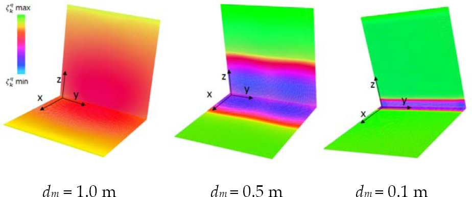
Finally, Fig. 12 shows a scenario where the tractor is driving on a trail with a ditch on the left side and high vegetation on the right side. The UPD interprets the scene, detecting correctly traversable ground and both positive and negative obstacles.

Figure 12.

Outdoor environment – (a) Original visual image. (b) RGB-D image obtained by the Bumblebee camera. (c) Estimation of the local normal vectors marked in red. (d) Results obtained from the UPD-based approach.

6. Conclusions

In this paper, a novel Unevenness Point Descriptor was described. It can be applied to 3D maps of the environment for traversability assessment. The proposed system is computationally simple and invariant to the orientation of the terrain. Thus, it is suitable for application to outdoor environments and specific cases including the presence of slopes or ramps that cannot be handled by other roughness indices proposed in the literature.

The UPD-based classifier was validated in both indoor and outdoor scenarios using an all-terrain rover and a test-bed tractor, showing good results. It could enhance vehicle mobility and safety through integration with localization, control and planning methods.

Footnotes

7. Acknowledgements

The financial support of the ERA-NET ICT-AGRI through the grant Ambient Awareness for Autonomous Agricultural Vehicles (QUAD-AV) is gratefully acknowledged.

References

Microsoft Xbox Kinect Sensor. [Online]. http://www.xbox.com/en-US/kinect

Asus Xtion Motion Sensor. [Online]. http://www.asus.com/Multimedia/Motion_Sensor/Xtion_PRO/.

Howard

and Saraji

, “Vision-Based Terrain Characterization and Traversability Assessment,” Journal of Robotic Systems, vol. 18, no. 10, pp. 77–587, 2001.

Milella

Reina

, and Siegwart

, “Computer vision methods for improved mobile robot state estimation in challenging terrains,” Journal of Multimedia, vol. 1, no. 7, pp. 49–61, 2006.

Reina

Underwood

Brooker

Durrant-Whyte

, “Radar-based Perception for Autonomous Outdoor Vehicles,” Journal of Field Robotics, vol. 28, no. 6, pp. 894–913, 2011.

Reina

Milella

, and Underwood

, “Self-learning classification of radar features for scene understanding,” Robotics and Autonomous Systems, vol. 60, no. 11, pp. 1377–1388, 2012.

Reina

Ishigami

Nagatani

and Yoshida

, “Odometry Correction Using Visual Slip-Angle Estimation for Planetary Exploration Rovers,” Advanced Robotics, vol. 24, no. 3, pp. 359–385, 2010.

Bogdan

R. B.

, “Semantic 3D Object Maps for Everyday Manipulation in Human Living Environments,” Technische Universitat Munchen, Munich, Germany, PhD Thesis 2009.

Iagnemma

and Dubowsky

, “Mobile Robots in Rough Terrain”, 2nd ed. Berlin, Germany: Springer, 2004.

10.

Osari

, “A new method for assessing land leveling to produce high quality consolidated paddy fields,” Paddy Water Environ, vol. 1, no. 1, pp. 35–41, 2003.

11.

Rohmer

Reina

and Yoshida

, “Dynamic Simulation-Based Action Planner for a Reconfigurable Hybrid Leg-Wheel Planetary Exploration Rover,” Advanced Robotics, vol. 24, no. 8-9, pp. 1219–1238, 2010.

12.

Reina

and Foglia

, “On the Mobility of all-terrain rovers”, Industrial Robot: An International Journal, vol. 40, no. 2, pp. 121–131, 2013.

13.

Point Grey. [Online]. http://www.ptgrey.com

14.

Reina

Milella

, “Towards Autonomous Agriculture: Automatic Ground Detection Using Trinocular Stereovision,” Sensors 2012, vol. 12, no. 9, 12405–12423, doi: 10.3390/s120912405.

15.

Cousins

and Rusu

R.B.

, “3D is here: Point Cloud Library (PCL),” IEEE International Conference on Robotics and Automation, Shanghai (China), 2011.

16.

Brandski

Thibaux

Hsu

Rusu

R. B.

, “Fast 3D Recognition and Pose Using the Viewpoint Feature Histogram,” in Proceedings of the 23rd IEEE/RSJ International Conference on Intelligent Robots and Systems (IROS), Taipei, Taiwan, 2010.

17.

Gross

Kobbelt

Pauly

, “Efficient Simplification of Point-Sampled Surfaces,” in Proceedings of the conference on Visualization, Washington, DC, USA, 2002.

18.

Marton

Z. C.

Blodow

Dolha

Beetz

Rusu

R. B.

, “Toward 3D Point cloud based object maps for household environments,” Robotics and Automation Systems, no. 56, pp. 927–941, 2008.

19.

Lowe

, “Distinctive Image Features from Scale-Invariant Key points,” International Journal of Computer Vision, vol. 2, no. 60, pp. 91–110, 2004.

20.

Berkmann

and Caelli

, “Computation of Surface Geometry and Segmentation Using Covariance Technique,” IEEE Transaction on Pattern Analysis and Machine Intelligence, vol. 16, no. 11, pp. 1114–1116, November 1994.

21.

Rouveure

Nielsen

Petersen

Reina

Foglia

Worst

Seyed-Sadri

Blas

M. R.

Faure

Milella

Lykkegård

, “The QUAD-AV Project: multi-sensory approach for obstacle detection in agricultural autonomous robotics,” International Conference of Agricultural Engineering CIGR-Ageng, 2012.

22.

Seraji

, “Traversability Index: A New Concept for Planetary Rovers,” in IEEE Intern. Conf. on Robotics and Automation, Detroit, MI, pp. 2006–2013, 1999.

Unevenness Point Descriptor for Terrain Analysis in Mobile Robot Applications

Abstract

Keywords

1. Introduction

2. System overview

3. Point feature representation

3.1 Normal estimation by Principal Component Analysis

4. Terrain analysis via normal vectors

4.1 Algorithm description

5. Experimental results

5.1 Case study 1: simulated data

5.2 Case study 2: indoor data

5.3 Case study 3: outdoor data

6. Conclusions

Footnotes

7. Acknowledgements

References