Applying Metaheuristic Algorithms for Output Rate Analysis in Two-Machine Robotic Manufacturing Cells

Abstract

This article analyses the output rate in two-machine flexible robotic manufacturing cells. The flexible CNC machines in this manufacturing cell can process different operations. The manufactured parts in the cell are identical and it is assumed that different operations are required to manufacture each part. Moreover, loading/unloading time of a part by the robot (ε), robot movement time between the machines and input and output areas (σ), and processing time of the j^th part on the machines (t_j) are considered to be fixed. The main objective of this article is to minimize cycle time in order to increase the output rate of the manufacturing cell. To achieve this goal, it is important to optimally assign operations required for manufacturing a part to each machine and to determine the optimal robot moves sequence. Accordingly, existing feasible movement policies in the cell and their cycle times have been reviewed, and then these policies have been considered in a new machine layout and their cycle times have been calculated based on the new robot moves sequence. Afterwards, a mathematical model has been presented to select optimal cycle time in the manufacturing cell and this model has been solved by a branch and bound exact algorithm; since the mathematical model is non-linear and the optimal solution cannot be obtained, two metaheuristic algorithms—genetic and simulated annealing algorithms—have also been proposed to solve the model and their results have been compared.

1. Introduction

A decisive factor in the modern competitive world of industry is time. Along with technological developments in industries and organizations, managers' decisions and their organizational activities and strategies have become very complicated; one of these strategies is to create an automation system in manufacturing organizations and industries; in this regard, a mechanical and programmable device named robot or manipulator is used to move parts between different stations. By arranging the machinery in a cell layout and using robots for automation of the process, managers minimize manufacturing time which leads to an increase in the efficiency of the production line or, in other words, an increase in manufacturing output in robotic manufacturing cells. Optimizing robot move sequencing which decreases manufacturing time of parts in robotic manufacturing cells has been a concern for researchers in recent years. There have been many studies on two-machine robotic manufacturing cells' scheduling. In most scheduling problems of robotic cells the objective function has been considered as a criterion; in single criterion scheduling just one objective function is used in the problem. One of the main single criterion functions used in previous studies is minimizing cycle time or, in other words, maximizing the output. Since the robot follows a computer program, there is a limited move sequence for it; to manufacture parts these movements are repeated. Therefore, because of its nature, robotic activities should be of a cyclic type and hence minimizing cycle time would be a related objective. Cycle time is the average necessary time to manufacture a part in a long run to the condition that each robot activity is repeated the same time.

The article by Sethi et al. [1] is considered to be the starting point for single criterion robotic cells' scheduling in literature. In this study, the objective was to maximize the output or, in other words, to minimize cycle time in a machine. One of the problems that this study deals with is how to produce similar parts by two machines. In another article, Sethi et al. [2] proved that the optimal solution of this problem is a one-unit cycle. Since in a two-machine cell there are two feasible one-unit cycles, they calculated the optimality range of each one of these cycles by comparing their processing times. Finding robot move sequencing in a one-unit cycle has been considered to minimize cycle time. A decision tree has been designed to find the optimal solution policy of one-unit cycles in a problem. Also, the number on one-unit cycles in an m-machine problem has been obtained as m!. Another main result of this article is the conjecture that one-unit cycles are more prominent than each n-unit (n≥2) cycle. Drobouchevitch et al. [3] have focused on the manner of manufacturing similar parts and have developed a formula for finding the number of cycles in a general m-machine cell. They illustrated that there are 52 cycles in an m-machine problem that can become one-unit feasible cycles; among these 13 cycles are dominant over the others. Sethi et al. [4] have looked on the manner of manufacturing different parts in two machines. With regard to fixed robot move sequencing in a two-machine cell and the appropriate manufacturing rate of different types of parts in MPS, they studied scheduling parts' entry into the entry station so that cycle time would decrease. In line with this they presented a polynomial time solvable algorithm to determine the optimum cycle. Logendran and Sriskandarajah [5] considered three kinds of different layouts in the two-machine scheduling problem that produces different parts and obtained the optimum robot move for these layouts. The problem of determining optimal robot move sequencing in non-identical parts manufacturing is like the two-machine no-wait flow shop problem and it is solved by the Gilmore–Gomory algorithm. Hurink and Knust [6] took the single-machine scheduling problem as a subset of the job-shop environment in which works are done by a robot among machines and they used a tabu search algorithm in the form of an extended travelling salesman problem to solve the problem. Their results illustrated that the tabu search algorithm calculates a good upper bound in a short time. Luan [7] investigated the robotic cell scheduling problem on two and three machines and by using a heuristic algorithm proved that there are two independent cycles in a two-machine robotic cell; also, using a genetic algorithm, he studied robotic cell scheduling on two machines in order to optimally assign the operation for each machine. Dawande et al. [8] studied throughput maximization in robotic cells with constant travel-time. Also Geismar et al. [9] considered productivity gains in flexible robotic cells. Deineko et al. [10] investigated a special mode of the two-machine flexible cell; in this study they assumed that the first machine does one activity and the second one performs k activities step by step. They transformed the scheduling problem in such a cell to a solvable case of the travelling salesman problem and they proposed a heuristic algorithm to solve it. Hall et al. [11, 12] devoted their study to the investigation of operation scheduling, robot move sequencing, cycle time study, complexity and simple modes of the problem. There are also some important review studies on robotic cell scheduling, including the extensive studies of Dawande et al. [13]. Recently, Gultekin et al. [14] have proposed a new robot move cycle in flexible robotic cells. In this study, they consider an m-machine robotic cell which is used for metal cutting operations. The proposed cycle here is called a pure cycle. In this cycle, the operation related to each part is done completely on only one machine and there is no part which is moved from one machine to another, rather it is carried from input buffer to one of the m-machines and from that machine to the output buffer. Each different sequence of loading and unloading operations leads to a different pure cycle. What is certain is the fact that two basic matters in robotic cell scheduling are robot move sequencing and part entry scheduling in the robotic cell; if in a robotic cell the purpose is to manufacture similar parts, the scheduling problem will be focused on determining optimal robot move sequencing. In the second part of this article the considered hypotheses are presented and movement policies in the proposed new cycle are described. In part 3, a mathematical programming model is presented to assign operations to the machines and determine robot move sequence and appropriate layout of machines' arrangement in robotic cells. In part 4, some algorithms for solving the presented mathematical model are suggested and computing results are analysed. Finally, in part 5, the conclusion and suggestions are presented.

2. Problem Definition

In this section, the considered hypotheses in this article regarding two-machine robotic cell scheduling are defined first. Then we have investigated the available policies of robot moves sequence in two-machine robotic cells; we have introduced a proposed new cycle for robot move sequencing and by regarding movement policies in the form of the new proposed cycle and layout we have calculated cycle time in the two-machine robotic cell.

2.1. Assumptions and Definitions

A two-machine robotic cell consists of a single gripper robot which is responsible for moving the parts and two machines which process the parts and are fed by this robot. In these manufacturing cells, machinery layout and arrangement, and robot movement can be performed in different ways. In this robotic cell it is assumed that each machine is capable of performing all operations and each part should be processed by both machines. The distance between each two successive points is considered equal or, in other words, robot movement time between each two successive places is equal; moreover, these movement times are additive. Also, it is assumed that loading and unloading time via robot is equal in all cases and the robot can move only one part at a time. The input buffer location is considered to be location zero; the first and second machines are located in the first and second place respectively, and the output location is considered to be the third location. In addition, in this study it is assumed that the machines in the robotic cell are identical.

Definition 1

An n-unit cycle means that the robot loads n parts into the cycle and for completing n parts, each job is exactly repeated n times and the robot finally returns to the initial state of the cycle.

Definition 2

A_ij activity means that the robot moves a part from location i to location j. In this article it is assumed that in the input area i = 0 in the location of the first machine i = 1, in the location of the second machine i = 2, and in the output area i = 3. It is also assumed that robot movement time between two successive locations is the same and equals S; the time of loading and unloading via robot in each location is also the same and equals ε.

Definition 3

n-unit cycle time (C_t): the necessary time to manufacture n parts in a cyclic process in a way that the robot begins from an initial state and in a specific sequence it performs the necessary operations to manufacture n parts and then it returns to the initial state.

Decision variables and parameters considered in this article are as follows:

• a:

  processing time of operations assigned to the first machine

• b:

  processing time of operations assigned to the second machine

• t_j:

  processing time of operation j on each machine

• ε:

  the time of part loading/unloading on machines in input/output areas by the robot

• δ:

  robot movement time between two successive locations

• w:

  robot waiting time in front of machines

• C_t:

  cycle time

• T_S1:

  cycle time of S₁ movement policy in robot linear move cycle

• T_S2:

  cycle time of S₂ movement policy in robot linear move cycle

• T_S12S21:

  cycle time of S₁₂S₂₁ movement policy in robot linear move cycle

• T_S1p:

  cycle time of S₁ movement policy in an arrangement like the new proposed cycle

• T_S2p:

  cycle time of S₂ movement policy in a settlement like the new proposed cycle

• T_S12S1p:

  cycle time of S₁₂S_21P movement policy in a settlement like the new proposed cycle

$\begin{array}{c}{X}_{1 j}=\{\begin{array}{l}1 If activity j is loaded on the first machine\\ 0 otherwise\end{array}\\ X_{2 j}=\{\begin{array}{l}1 If activity j is loaded on the second machine\\ 0 otherwise\end{array}\end{array}$

2.2. Investigating the Existing Feasible Movement Cycles in Two-machine Robotic Cell

In these cycles it is assumed that the robot has a linear movement on a rail and the machines and input and output areas are located in front of it; according to Crama and Klundert's study [15] this layout is illustrated in fig. 1.

Figure 1.

Linear layout in a two-machine

Akturk et al. [16] have assumed that the machines are flexible, i.e., they are capable of doing all operations needed to produce a part; they have also assumed that robotic cells are flexible and the processing time of one operation by both machines is the same, in other words, it is assumed that the machines are identical and the time of loading/unloading (ε) by the robot is equal and robot movement time between two successive locations (δ) is also equal. Citing Sethi et al.‘s article [2] they have introduced S₁, S₂, S₁₂S₂₁ movement policies as the following; each cycle time is also calculated and analysed.

S₁ movement cycle

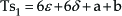
In accordance with the presented definitions in this article, in this cycle the robot move sequence is A₀₁ A₁₂ A₂₃ where in a two-machine robotic cell location zero is related to input area, location one is for machine one, location two for the second machine and location three is related to output area. According to the defined movements, S₁ cycle is a one-unit cycle and its cycle time is defined as Eq. (1). In the beginning of this cycle there are no parts on the machines and the robot is in front of the input area.

$T{s}_1=6\epsilon + 6\delta +a + b$

(1)

S₂ movement cycle

In this cycle the robot move sequence is A₀₁ A₂₃ A₁₂. At the beginning of this cycle there is one part on the second machine and the robot is in front of the input area, and after performing the mentioned movements it returns to the input area. The time of this cycle has been calculated like Eq. (2). This cycle is also a one-unit cycle

$T{s}_2=6\epsilon + 8\delta +Max \left\{0 , w_1 , w_2 \right\}$

(2)

$w_1= a - (2\epsilon + 4\delta )$

(3)

$w_2= b - (2\epsilon + 4\delta )$

(4)

S₁₂ S₂₁ movement cycle

In this cycle the robot move sequence is A₀₁ A₁₂ A₀₁ A₂₃ A₁₂ A₁₃. At the beginning of this cycle both machines are empty and the robot is in front of the input area, and after performing the above mentioned movements it returns to the input area; this cycle is a two-unit cycle. The time for manufacturing a part in this cycle is calculated as Eq. (5).

$T_{S_{12} S_{21}}=6 \epsilon + 7 \delta +\raisebox{1ex}{$(a+b)$}\!\left/ \!\raisebox{-1ex}{$2$}\right.+\frac{1}{2}Max \left\{ 0 , w_1 , w_2 \right\}$

(5)

$w_1= a - (2\epsilon + 4\delta )$

(6)

$w_2= b - (2\epsilon + 4\delta )$

(7)

2.3. Investigating the Available Movement Cycles in the New Layout Design

In the new cycle the assumption that the robot movement is linear is removed and it is assumed that the robot is located between two machines and input and output areas are located at one side of the robot close to each other and the robot has a rotating movement. Fig.2 illustrates the layout design of this proposed cell.

Figure 2.

Layout design of the new cycle

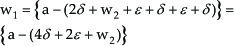
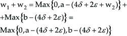
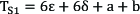
In this proposed robotic cell it is assumed that the input and output areas are beside each other and the space between them is trivial as compared to the space between the two machines and the machines and input and output areas; robot movement time between the input and output area is also trivial in a way that it can be ignored and the input and output area can be taken as a single place. Considering movement sequence in S₁₂ S₂₁, S₂, S₁ cycles which are presented in section 2.2 and also the layout design of the proposed robotic cell in section 2.3, one can consider the sequence of the above mentioned movements according to existing policies in robot movement via the proposed layout design in a way that one can investigate the same movement sequence on the new robotic cell in which the robot has only one rotating movement and compare their related cycle times. For more information about this movement sequence one can refer to Sethi et al.‘s article [2]. In this way, according to these movement policies, in the following parts the cycle times of S₁₂S₂₁,S₂,S₁ movement policies are illustrated as T_{S12 S21p}, T_S2p,T_S1p respectively and their related cycle times are calculated as follows:

S_1p Cycle time

$\begin{array}{l}{T}_S{}_{1p} =\epsilon +\delta +\epsilon +a+\epsilon +2\delta +\epsilon +b+\epsilon +\delta +\epsilon =\\ 4\delta +6\epsilon +a+b\end{array}$

(8)

S_2p Cycle time

$\begin{array}{l}{T}_S{}_{2p} =\epsilon +\delta +\epsilon +2\delta +w_2+\epsilon +\delta +\epsilon +\\ +\delta +w_1+\epsilon +2\delta +\epsilon +\delta =\\ 8\delta +6\epsilon +w_1+w_2\end{array}$

(9)

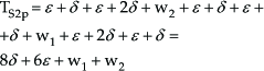
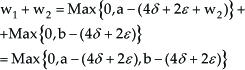
In which the waiting time of the robot in front of two machines is calculated as Eq. (10), Eq. (11)

$\begin{array}{l}{w}_1=\left\{ a-(2\delta +w_2+\epsilon +\delta +\epsilon +\delta )\right\}=\\ =\left\{ a-(4\delta +2\epsilon +w_2)\right\}\end{array}$

(10)

$w_2=\left\{ b-(\delta +\epsilon +\delta +\epsilon +2\delta )\right\}=\left\{ b-(4\delta +2\epsilon )\right\}$

(11)

$\begin{array}{l}{w}_1+w_2=Max\left\{0,a-(4\delta +2\epsilon +w_2)\right\}+\\ +Max\left\{0,b-(4\delta +2\epsilon )\right\} \\ =Max\left\{0,a-(4\delta +2\epsilon ),b-(4\delta +2\epsilon )\right\}\end{array}$

(12)

As a result S_2p cycle time is calculated as Eq. (13)

$T_S{}_{2p} =8\delta +6\epsilon +Max\left\{0,a-(4\delta +2\epsilon ),b-(4\delta +2\epsilon )\right\}$

(13)

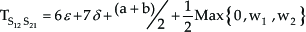
S_12pS_21p cycle time

$\begin{array}{l}\begin{array}{l}{\mathrm{T}}_{\mathrm{S}12\mathrm{S}21\mathrm{p}}=\varepsilon +\delta +\varepsilon +\mathrm{a}+\varepsilon +2\delta +\varepsilon +\delta +\varepsilon +\delta +\varepsilon +2\delta +{\mathrm{w}}_2\\ +\varepsilon +\delta +\varepsilon +\delta +{\mathrm{w}}_1+\varepsilon +2\delta +\varepsilon +\mathrm{b}+\varepsilon +\delta +\varepsilon \end{array}\hfill \\ \hspace{0.17em}\hspace{0.17em}\hspace{0.17em}\hspace{0.17em}\hspace{0.17em}\hspace{0.17em}\hspace{0.17em}\hspace{0.17em}\hspace{0.17em}\hspace{0.17em}\hspace{0.17em}\hspace{0.17em}\hspace{0.17em}\hspace{0.17em}\hspace{0.17em}{\mathrm{T}}_{2-\text{unitS}12\mathrm{S}21\mathrm{p}}=12\delta +12\varepsilon +\mathrm{a}+\mathrm{b}+{\mathrm{w}}_1+{\mathrm{w}}_2\hfill \end{array}$

(14)

Where the robot waiting time in front of two machines is as Eq. (15), Eq. (16)

$\begin{array}{l}{w}_1=\left\{ a-(2\delta +w_2+\epsilon +\delta +\epsilon +\delta )\right\}=\\ \left\{ a-(4\delta +2\epsilon +w_2)\right\}\end{array}$

(15)

$\begin{array}{l}{w}_2=\left\{ b-(\delta +\epsilon +\delta +\epsilon +2\delta )\right\}=\\ \left\{ b-(4\delta +2\epsilon )\right\} \end{array}$

(16)

$\begin{array}{l}{w}_1+w_2=Max\left\{0,a-(4\delta +2\epsilon +w_2)\right\}+\\ +Max\left\{b-(4\delta +2\epsilon )\right\} =\\ Max\left\{0,a-(4\delta +2\epsilon ),b-(4\delta +2\epsilon )\right\}\end{array}$

(17)

As a result S₁₂S₂₁ cycle time for a part is calculated as Eq. (18)

$\begin{array}{l}{T}_S{}_{12 S21p} =6\delta +6\epsilon +\frac{a}{2}+\frac{b}{2}+\\ \frac{1}{2} Max\left\{0,a-(4\delta +2\epsilon ),b-(4\delta +2\epsilon )\right\} \end{array}$

(18)

3. The Proposed Mathematical Model

In the previous section the existing movement policies in two-machine robotic cells were presented and then in the form of arranging in a new layout these policies were investigated again. The cycle time of each proposed movement cycles was calculated. Based on some special assumptions one can compare cycle times in linear robot movement with that in the new approach. Akturk et al. [16] have performed parametric analysis to compare the existing movement policies of a two-machine robotic cell; they have presented optimal movement cycles in different cases. In this article, as the operation's processing time related to each part, loading/unloading time, and robot movement are obvious, we propose a mathematical model whose purpose is to determine the best movement policy and layout design type of robotic cell by assigning operations to the machines. With regard to Eq. (2), Eq. (13), cycle time in both cases (linear movement and rotating movement of the robot) is equal. Therefore, only one of these movement cycles is considered in the presented model and decision making about using an appropriate layout design is based on production line overview. The problem's assumptions, indices, parameters and decision variables are as follows:

Assumptions

In this section the assumptions related to scheduling problem with the condition that the cell is flexible are defined as follows:

1. If a job begins on a machine, it will remain on the same machine until it is finished. In other words, no pre-emption is allowed.

2. If an operation begins on a machine, no other operation can replace it until it is finished, unless preemption allowed for the problem.

3. The machines cannot be idle during operations.

4. No machine fails in the operation process; they are all available during the schedule.

5. All the machines are identical and the processing time of an operation is the same on each machine.

6. There is a holder arm (robot) in a robotic cell.

7. Robotic cell system is flexible, i.e., it can simultaneously process several operations.

8. Loading/unloading time (ε) by the robot is the same; robot movement time between two successive locations (δ) is also the same.

9. Production is cyclic.

10. The problem is a flow shop problem.

11. Production policy is the same for all parts.

12. The robot cannot reload a loaded machine.

13. The robot cannot unload an idle machine.

14. All the jobs are equally valuable and all of them should complete their process.

15. Machines' set up time for different jobs can be ignored.

16. The input and output areas are beside each other and the space between them is trivial as compared to the space between the two machines and the machines and input and output areas in a way that by ignoring the movement time between input and output area they can be taken as a single place.

17. The robot has a rotating movement.

Indices

i: job related indices (i=1,…,n)

Parameters

n: number of jobs

t_i: i^th job/operation processing time

a: sum of the processing times related to the operations assigned to the first machine

b: sum of the processing times related to the operations assigned to the second machine

Decision variables

$\begin{array}{c}{X}_{1 j}=\{\begin{array}{l}1 If activity j is loaded on the first machine\\ 0 otherwise\end{array}\\ X_{2 j}=\{\begin{array}{l}1 If activity j is loaded on the second machine\\ 0 otherwise\end{array}\end{array}$

With regard to the considered parameters and variables, if it is assumed that in both the linear movement and rotating movement of the robot loading/unloading time (ε) and robot movement (δ) are equal and if the machines are considered identical in both cases, the mathematical model of the problem to determine optimal movement policy and the method to assign the operations to the machines will be as follows:

$MIN Z=C$

(19)

$C=MIN\left({\mathrm{T}}_{\mathrm{S}1},{\mathrm{T}}_{\mathrm{S}2},{\mathrm{T}}_{\mathrm{S}12\mathrm{S}21},{\mathrm{T}}_{\mathrm{S}1\mathrm{P}},{\mathrm{T}}_{\mathrm{S}12\mathrm{S}21\mathrm{P}}\right)$

(20)

$\mathrm{W}=\text{MAX}\left\{0,\mathrm{a}-\left(2\text{ε}+4\text{δ}\right),\mathrm{b}-\left(2\text{ε}+4\text{δ}\right)\right\}$

(21)

$a=\sum _{i=1}^n{x}_{1i}\times t_i$

(22)

$b={\displaystyle \sum }_{i=1}^n{x}_{2i}\times t_i$

(23)

$x_{1i}+x_{2i}=1 \forall i$

(24)

${\mathrm{T}}_{\mathrm{S}1}=6\text{ε}+6\text{δ}+\mathrm{a}+\mathrm{b}$

(25)

${\mathrm{T}}_{\mathrm{S}2}=6\text{ε}+8\text{δ}+\mathrm{W}$

(26)

${\mathrm{T}}_{\mathrm{S}12\mathrm{S}21}=6\text{ε}+7\text{δ}+\frac{\mathrm{a}}{2}+\frac{\mathrm{b}}{2}+\frac{\mathrm{W}}{2}$

(27)

${\mathrm{T}}_{\mathrm{S}1\mathrm{P}}=6\text{ε}+4\text{δ}+\mathrm{a}+\mathrm{b}$

(28)

${\mathrm{T}}_{\mathrm{S}12\mathrm{S}21\mathrm{P}}=6\text{ε}+6\text{δ}+\frac{\mathrm{a}}{2}+\frac{\mathrm{b}}{2}+\frac{\mathrm{W}}{2}$

(29)

$x_{1\mathrm{i}},x_{2\mathrm{i}}\in \left\{0,1\right\} \forall i$

(30)

In the presented model, Eq. (19) and Eq. (20), the model's objective function, choose the minimum cycle time which is to choose the minimum time among S₁,S₂,S₁₂ S₂₁,S_1p,S₁₂S_21p movement cycles.

Eq. (21) determines waiting time in the cycle according to δ,ε constant parameters and different a,b.

Eq. (22) determines the processing time on the first machine according to the operations assigned to the first machine.

Eq. (23), like Eq. (22), determines the processing time of the operations assigned to the second machine.

Eq. (24) confirms the matter that in the manufacturing of one part each necessary operation to produce that part is assigned only to one machine.

Eq. (25) illustrates S₁ cycle time for robot linear movement.

Eq. (26) illustrates S₂ cycle time for robot linear movement.

Eq. (27) illustrates S₁₂S₂₁ cycle time for robot linear movement.

Eq. (28) illustrates S_1p cycle time for robot rotating movement.

Eq. (29) illustrates S₁₂S_21p cycle time for robot rotating movement.

Eq. (30) illustrates that X_1i, X_2i decision variables are binary.

As observed, the proposed model has t_j,δ,ε input parameters which are assumed to be constant while solving the problem; the values of these three parameters can change according to the physical characteristics of the manufacturing cell and the part which is going to be manufactured in this cell. Like the problem of assigning the operations in S₃ cycle in a three-machine robotic manufacturing cell [17], [12] the proposed model is an NP-hard problem. By assigning different operations to the first and second machines, and obtaining different values of a, b, w, this model tries to determine the optimal cycle time and robot movement policy.

4. Problem Solution

For solving the proposed model in this article, in addition to exact solution methods, simulated annealing and genetic algorithms are also used.

4.1. Genetic Algorithm

This algorithm is the most famous evolutionary algorithm; its overall structure is as follows:

A solution structure is first defined to show the problem's solutions. Using this structure the primary generation of solutions is randomly created by a predefined population size. The primary chromosomes which are produced are called parent chromosomes and their number is equal to the generation/population size. The size of each generation/population in the genetic algorithm is fixed. Then the repetitive loop of the algorithm begins. In each run of this loop, chromosomes and genes that have the necessary condition for crossover and mutation are selected, and crossover and mutation operators are applied on them. As a result of this process new chromosomes (offspring/children) are generated. Chromosomes of the produced child via crossover and mutation operators together with parent chromosomes of the previous generation/population create pool chromosomes; the size of pool chromosomes is certainly bigger than the chromosomes of the previous generation. So the next generation/population is selected from pool chromosomes. Then the stop condition is investigated; if the condition holds, the algorithm will end and the best chromosome of the last generation will be selected as the best answer, otherwise, another repetition of the algorithm will be performed.

The main components of genetic algorithms are as follows:

• Coding

• Generating primary population

• Determining fitness

• Operators of genetic algorithm

• Selection process

• Algorithm's parameter values

In this paper, the needed components to solve the model are defined as follows:

4.1.1. Coding

The first stage of genetic algorithm is to structure decision variables (coding). The structure of decision variables is often illustrated by a vector or matrix; each item of this vector or matrix is one decision variable. The structure of decision variables in a genetic algorithm is called chromosome and each item of a chromosome is called gene. In this article, the following vector chromosome structure has been used (fig.3):

Figure 3.

Solution structure

It should be clarified that the number of genes in the proposed chromosome equals n which is the same as the number of jobs/operations. As described in the body of the article, processing a part of jobs/operations related to each manufacturing part is performed by machine 1 and the rest is performed by machine 2. Gene values in this chromosome (r_j), j= 1, …, n, refers to the number of machine on which the processing operation of job j related to the manufacturing part is performed. Therefore, r_j = 1 if processing of job j is performed by machine 1 and r_j = 2 if it is performed by machine 2. After the structure of the chromosome was determined, the primary solution is randomly generated.

4.1.2. Generating the Primary Population

The collection of chromosomes is called population. Instead of focusing on one solution (chromosome), the genetic algorithm works on a collection of chromosomes. Population size reveals the number of chromosomes in each generation.

4.1.3. Fitness

The value of objective function according to each chromosome is called fitness of that chromosome.

4.1.4. Genetic Algorithm Operators

In a genetic algorithm, the approaches that are performed on one or more chromosomes and generate one or more new chromosomes (children) are called genetic operators. The most important genetic operators are crossover and mutation.

• Crossover operator: this operator is applied on a pair of chromosomes and generates one or more chromosomes. In this article, a one-point-cut crossover operator has been used. To implement one-point-cut crossover, two parent chromosomes P₁,P₂ are first considered and then the cut point is randomly selected from the end points of genes 1 to n-1 of these chromosomes. Assume that when chromosomes' cut points are at the end of k^th gene, the genes before the cut point in chromosome P₁(r₁ – r_k) are moved into corresponding places in the first child chromosome (CH₁)) and other genes of the first child chromosome (CH₁) are filled with the genes after the cut point of chromosome P₂(r_k+1 - r_n). In the same manner, the genes before the cut point in parent chromosome P₂₍r₁ – r_k)are moved to corresponding places in the second child chromosome (CH₂) and the genes after cut point in parent chromosome P₁ (r_k+1-r_n)are moved to corresponding places in the second child chromosome(CH₂). Figure 4 illustrates a one-point-cut crossover.

• Mutation operator: this operator is applied on one chromosome and changes one or more genes on it so that a new chromosome is generated. The primary chromosome is called parent and the new one is called offspring. To apply the mutation operator in this article, one gene is randomly selected at first, then the gene's value is changed in a way that the generated chromosome is feasible. Fig. 5 illustrates the method of applying the mutation operator on a chromosome.

Figure 4.

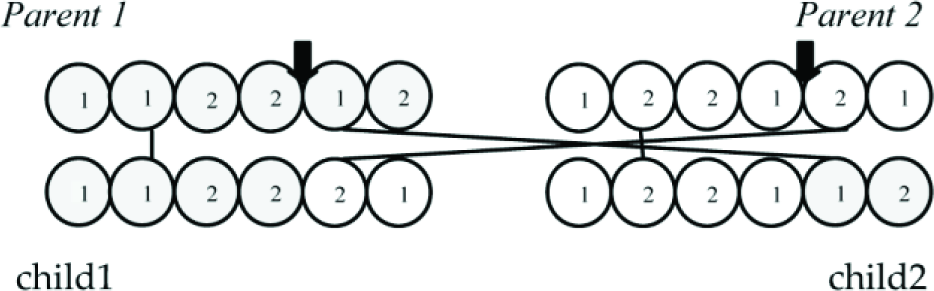
The method of applying the crossover operator on two parent chromosomes

Figure 5.

The method of applying the mutation operator on one chromosome

4.1.5. Selection Process

In this article, a mixed or combined strategy has been used to select new generation chromosomes; in this way, a percentage of the best pool chromosomes are placed in the new generation and then the remaining chromosomes of the next generation are selected randomly from pool chromosomes.

4.1.6. The Value of Algorithm Parameters

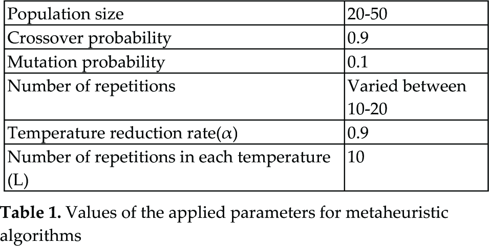
The necessary parameters for run of genetic algorithm are population size, crossover probability, mutation probability and the number of generations. The number of repetitions is based on the problem size. In setting the parameters one should be careful that there is a balance between the algorithm's running time and the quality of solutions. Values of the applied parameters of genetic algorithm have been determined in table 1.

Table 1.

Values of the applied parameters for metaheuristic algorithms

Population size	20-50
Crossover probability	0.9
Mutation probability	0.1
Number of repetitions	Varied between 10-20
Temperature reduction rate(α)	0.9
Number of repetitions in each temperature (L)	10

4.2. Simulated Annealing Algorithm

A simulated annealing algorithm (SA) is inspired by the process of metals annealing. In a real annealing process, the metal's temperature is increased to a point that all the molecules are scattered in a molten form, then temperature will slowly decrease. Temperature decrease in real annealing is like decreasing the value of objective function for minimization problems. As the temperature decrease rate in real annealing affects the quality of the final material, the temperature decrease rate in an SA algorithm also affects the quality of the final solution. One characteristic of the SA algorithm is that it accepts non-improving solutions; this causes the algorithm not to get captured at a local optimum. This algorithm begins with a primary random solution; then in each temperature some of the primary solution neighbourhoods are studied. If the objective function's value of the neighbour's solution is better than the objective function's value of the primary solution, the neighbour's solution will be accepted, otherwise, to escape the local optimum the neighbour's solution with probability of $exp\left(-\frac{\mathrm{\Delta }}{T}\right)$ will be accepted. This process will be repeated until a predefined number of neighborhoods are studied in each temperature. Afterwards the temperature will decrease; the predefined number of neighbourhood is also studied in this new temperature. The algorithm will stop when it reaches the stopping criterion. The pseudo-code of simulated annealing algorithm is illustrated in Fig.6.

Figure 6.

Pseudo-code of SA algorithm for minimization problems [18]

The basic parameters of the SA algorithm are as follows:

4.2.1. Initial Temperature

The initial temperature is one of the basic parameters of the SA algorithm. The initial temperature should be selected in a way that most of the non-improving solutions are accepted in the first repetition. In this article, the following heuristic method has been used to determine the initial temperature. The pseudo-code of the initial temperature is illustrated in Fig. 7.

Figure 7.

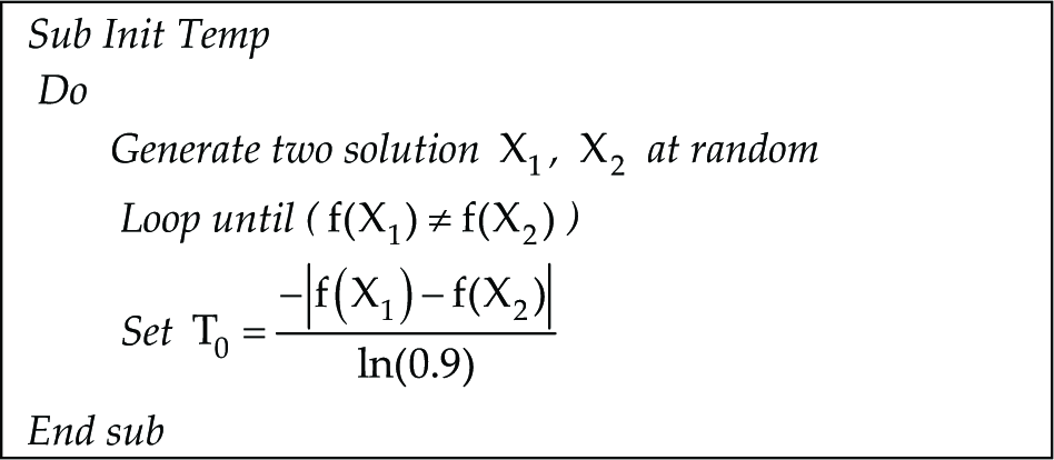
Pseudo-code determining the initial temperature of the SA algorithm [19]

4.2.2. Temperature Decrement Rule

The SA algorithm begins with a relatively high temperature which decreases slowly on each repetition. There are various methods to reduce temperature in each repetition; in this article, geometric scheduling criterion has been used:

$T_k=\alpha T_{k-1} 0<\alpha <1$

(31)

In the above relation, T_k is the system's temperature in the k^th repetition and α is the temperature reduction rate. Selecting a large value for α results in slow temperature decrement and better solution space searching, on the other hand, it increases the algorithm's run time. Selecting a small value for α results in fast temperature decrement and fast solution space searching. Therefore, α value should be selected in such a way that there will be a balance between the algorithm's run time and the quality of solutions. In this paper, α value has been considered to be 0.9.

4.2.3. Neighbourhood Structure

Neighbour solutions are a set of feasible solutions which are obtained from the primary solution. Each neighbour solution can be obtained through one movement (a change in the present solution). In this article, the following neighbourhood structure has been used; in this structure one of the genes is randomly selected and then its value is changed in a way that the resulted solution will be feasible. Neighbourhood structure is illustrated in Fig. 8.

Figure 8.

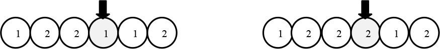
Neighbourhood structure

4.2.4. Number of Repetitions in Each Temperature (L)

This parameter controls the number of investigated neighbourhoods in each temperature. L value should be selected large, to the extent that it results in an effective neighbourhood search. On the other hand, L value should not be so large that it would result in an ineffective search and increased run time. In this paper, the number of repetitions in each temperature (L) has been considered to be 10.

4.2.5. Stopping Criterion

In the presented algorithm, the stopping criterion has been considered to be the final temperature. The final temperature should be selected in a way that the probability of accepting non-improving solutions in the final repetitions will be close to zero.

4.3. Numerical Examples

In this section, ten numerical examples are solved to evaluate the presented model. The early examples have a small scale, but it increases regularly in such a way that the final examples have a large scale. The processing time of each job has been obtained through the following simulation approach:

Processing time of each job (second): uniform distribution

$\begin{array}{c}\mathrm{U}~\left[\begin{array}{ll}10\hfill & 200\hfill \end{array}\right]\\ \varepsilon :\mathrm{U}~\left[\begin{array}{ll}1\hfill & 5\hfill \end{array}\right],\delta :\mathrm{U}~\left[\begin{array}{ll}3\hfill & 15\hfill \end{array}\right]\end{array}$

Each one of these problems have been solved by LINGO 8.0 software at first. LINGO 8.0 is able to produce local optimal solutions for nonlinear problems. Therefore, metaheuristic algorithms should be used for solving this problem. The presented metaheuristic algorithms(GA,SA) have been encoded by MATLAB 7.0 and have been implemented via a PC with 2.4 GHZ of CPU and 4 Gb of RAM. A summary of parameter values necessary to implement the presented genetic and simulated annealing algorithms are displayed in table 1. It should be noted that the size of population has been considered to be 20-50 chromosomes relative to problem size. The population size in sample problems 1, 2, and 3 which are small size problems has been considered to be 20; in problems 4, 5, 6, and 7 it is 35 and in problems 8, 9 and 10 it is 50. Also, for suitable diversification and intensification in solution search related to sample problems, crossover and mutation probabilities have been considered to be 0.9 and 0.1 respectively.

The results of solving the sample problems by LINGO 8.0 and GA and SA algorithms are illustrated in tables 2 and 3. Each sample problem 1-10, which has been solved through GA and SA, has been run 10 times; in fact, the results illustrated in table 3 are the data related to the best, the worst, and the average value of objective function and the average runtime for solving each problem in 10 runs, and the solution of that problem by GA and SA.

Table 2.

The values of the objective functions obtained via LINGO 8.0

Problem No.	Number of jobs	Best OFV	BOUND	run time (second)
1	5	2.949.993	2.949.993	0
2	10	651	651	0
3	15	738	738	0
4	20	1149	1149	0
5	25	1.579.998	1.579.998	0
6	30	1503	1503	0
7	35	1858	1858	1
8	40	1921	1921	1
9	45	2.713.997	2.713.997	1
10	50	2.653.998	2.653.998	0

OFV=Objective Function Value

Table 3.

The values of the objective functions obtained via metaheuristic algorithms

Problem No.	Number of jobs	algorithm	Best OFV	Worst OFV	Average OFV	Average running time (second)
1	5	GA	242	242	242	0.0624
		SA	242	303	266.4	2.0155
2	10	GA	613	614	613.8	0.0405
		SA	613	618	614.8	6.0653
3	15	GA	735	738	735.6	0.05304
		SA	735	735	735	2.1298
4	20	GA	770	776	771.2	0.05304
		SA	770	772	770.6	2.5334
5	25	GA	1570	1571	1570.4	0.0998
		SA	1570	1571	1570.4	4.9202
6	30	GA	1503	1503	1503	0.1903
		SA	1503	1505	1504	5.7314
7	35	GA	1857	1857	1857	0.1934
		SA	1857	1857	1857	5.0450
8	40	GA	1920	1921	1920.6	0.1716
		SA	1920	1921	1920.2	8.2025
9	45	GA	2479	2480	2479.6	0.1684
		SA	2479	2481	2479.4	7.6690
10	50	GA	2518	2518	2518	0.1872
		SA	2518	2518	2518	9.4880

OFV=Objective Function Value

5. Conclusion and Suggestion

In this article a new approach has been used to find the optimum cycle time and move sequence, and to determine optimal robot movement policies in two-machine robotic manufacturing cells. By presenting the proposed layout design in the form of the existing feasible movement policies for robot linear movement sequences, the problem has been formulated in the form of a mathematical programming model. In addition, for solving the proposed model, two metaheuristic algorithms named GA and SA algorithms have been presented and the obtained results from these algorithms have been compared with deterministic solutions of the problem. The results illustrate that although the model has a high computational complexity, the presented metaheuristic algorithms have produced a high quality solution in an acceptably short time. Also, the GA algorithm as compared to the SA algorithm has obtained high quality results in less time. In the following studies the problem will be extended to a robotic manufacturing cell which produces different parts and the obtained results from this problem will be analysed.