Sage Journals: Discover world-class research

Abstract

Flexible robotic cells are used to produce standardized items at a high production speed. In this study, the scheduling problem of a flexible robotic cell is considered. Machines are identical and parallel. In the cell, there is an input and an output buffer, wherein the unprocessed and the finished items are kept, respectively. There is a robot performing the loading/unloading operations of the machines and transporting the items. The system repeats a cycle in its long run. It is assumed that each machine processes one part in each cycle. The cycle time depends on the order of the actions. Therefore, determining the order of the actions to minimize the cycle time is an optimization problem. A new mathematical model is presented to solve the problem, and as an alternative, a simulated annealing algorithm is developed for large-size problems. In the simulated annealing algorithm, the objective function value of a given solution is computed by solving a linear programming model which is the first case in the literature to the best of our knowledge. Several numerical examples are solved using the proposed methods, and their performances are evaluated.

Keywords

Flexible manufacturing robotic cell cyclic scheduling meta-heuristics

Introduction

Cell manufacturing indicates a connective system among product-oriented and process-oriented systems. Using a robot in such cells helps to produce standardized items at a high production speed.¹ A cell with a number of computer numerical control (CNC) machines and a robot is called flexible robotic cell (FRC).² In FRCs, the CNC machines perform manufacturing processes, and the robot transports the items from the input buffer to the machines, loads/unloads the CNC machines, and transports the items to the output buffer.³ The same group of processes is performed on all the CNC machines. Hence, each item is processed only on one machine. The considered system repeats a cycle in its long run. If the system is in a specific state at the beginning of a cycle, it reaches the same state at the end of the cycle and then repeats the same actions in the same order in the subsequent cycles. The duration of a cycle is called cycle time. Each machine processes one part in each cycle. Decreasing the cycle time in such a system means increasing the production rate. The cycle time depends on the order of the actions. Thus, determining the order of the actions to minimize the cycle time is an optimization problem.

A thorough review of inflexiable robotic cell scheduling problem with single and multiple robots including a single and dual gripper can be found in the survey by Dawande et al.⁴ Gultekin et al.⁵ suggested a new cycle for FRC that performs better in comparison to the classical robot move cycles for two-machine cells. Moreover, they showed that a robot-centered layout reduces the cycle time compared to an in-line layout and found an optimal number of machines to minimize the cycle time of m-machine cells. In another study, Gultekin et al.⁶ presented a mathematical formulation to determine the minimum cycle time for a parallel machine cell. Jolai et al.⁷ studied an FRC scheduling problem with identical part types, machines are flexible and able to swap. They determined all one-unit cycle times and proposed a new sequence of robot movements that dominates all robot move cycles. Yildiz et al.⁸ proposed two pure cycles and showed that these two cycles jointly dominate all other pure cycles for a broad range of the process times. They also presented the worst case for minimizing the cycle time. Foumani and Jenab⁹ developed one-unit cycles for line layout robotic cells and presented a robot move sequence that minimizes the cycle time. They also introduced the optimality regions when all parts met the first machine twice and determined the optimality conditions for different cycles when each part meets both machines twice. They carried out the sensitivity analysis for both cases and suggested the best and the worst cycles mathematically. Foumani and Jenab¹⁰ extended their research to m-unit pure cycles when the robot is able to swap. They presented a lower bound and introduced a pure cycle that always dominates the others. Jiang et al.¹¹ applied two heuristics to minimize the makespan of a job scheduling problem. They considered a two-machine system where the machines are parallel and identical, and the machines are loaded/unloaded by a server. Gultekin et al.¹² studied on an FRC in which a dual-gripper robot serves the machines. They considered a two-machine FRC and found five feasible pure cycles to maximize the throughput rate. Foumani et al.¹³ focused on maximizing the throughput rate of FRC problems including multi-function robotic cells, and in another study, they considered the scheduling problem of n-unit production in the FRC and found that one-unit cycles dominate the rest. Furthermore, they considered an FRC including two machines with three different scenarios of inspections including in-process and post-process inspection, the cell with a multi-function robot, and the linear layout FRC.¹⁴ They extended their studies on two-machine FRCs considering different pick-up scenarios. They converted a multiple sensor system to a single sensor and found the cycle times based on a geometric distribution.¹⁵

Recently, simulated annealing algorithm (SAA) is used to solve a wide range of optimization problems. SAA is prominence from high solution performance, fine results in short times among meta-heuristics approach. In the literature, the SAA has been used for solving the traveling salesman problem (TSP),¹⁶ the location-routing problem,¹⁷ the emergency logistics problem,¹⁸ the assembly line balancing problem,^19,20 disassembly scheduling problem,²¹ the production and preventive maintenance problem,²² the flow shop scheduling problem,²³ the clustering problem,²⁴ the facility layout problem,²⁵ the cell formation problem,²⁶ for distributed job shop problem,²⁷ and so on.

In the literature, some researchers employed TSP approaches for modeling scheduling problem of the FRC with m-machine and a robot. As examples, Foumani et al.²⁸ formulated the FRC problem including a multi-function robot, as a TSP aimed to minimize the cycle time or to maximize the production rate. Additionally, to calculate the productivity of the cell, they found the lower bound for the objective function considering the both uphill and downhill permutations. Gultekin et al.⁶ developed a mathematical model for the scheduling problem of FRC considering fixed process time for the machines using TSP’s Miller–Tucker–Zemlin (MTZ) method and expressed that the problem is non-deterministic polynomial-time (NP)-hard. They used CPLEX 9.0 and reported some evidence for solving the problem considering four, five and six machines in the cell. Similar to any other type of NP-hard problems, computational time for solving the problem exponentially rises in case the number of the machines in the cell is increased.²⁹ Using twenty random inputs, they concluded that the computational time for the cell with four-machine is 7.72, for the five-machine case is 1866.7 and with only a single run for a six-machine case, it needs 805,184.4 s to solve the problem. They did not use any meta-heuristic algorithm for solving large-sized problems. In their model, they faced with a non-linear constraint (i.e. constraint 4) and in order to propose a linear model, they defined a new auxiliary variable, namely, Y_lUj and six extra liner constraints (i.e. constraints 9–14) to convert the non-linear model to a linear one. Y_lUj and its related constraints have a notable adverse effect on computational time (performance) of the model especially for the FRC with more machines. These issues motivated the authors to model the problem using other exist TSP based modeling approaches along with considering variable process time for the machines. Since, the scheduling is more vital and complicated for the cells with short process time in the machines or for the cells with a busy robot (the machines have idle time, and robot activity order determine the cycle time), and also aiming to employ fewer number of variables and constraint in the model, “Network Flow” modeling approach is used.³⁰ For solving the scheduling problem of large-size cells a more feasible model from computational time points of view is needed. In addition, the use of a powerful meta-heuristic algorithm from time complexity, space complexity, the advantages and disadvantages of the calculation results is essential.

In this article, TSP’s “Network Flow” modeling approach is used to model the scheduling problem of FRC with m-machine. Moreover, SAA is examined to solve the large-size problem in the model. For doing this, first, a new mathematical model for the scheduling problem is proposed; next, for justification of the proposed model, the developed model and an existing model in the literature are solved by CPLEX under normalized conditions, and the results are compared. Finally, SAA is used to solve the large-sized problem and performances of the proposed approach using several numerical instances.

The considered problem is defined and formulated in section “Problem definition and formulation.” Section “The developed SAA” describes the proposed SAA. Section “Experimental results” includes experimental results about the performance of the proposed methods. The study is concluded in section “Conclusion.”

Problem definition and formulation

A schematic of an FRC can be seen in Figure 1. Let the number of the machines in the considered FRC-explained in the introduction be m. The process time of a part on a machine is p. (In the rest of the article, the machines are assumed to be identical. Thus, they have the same process time p. In the case of non-identical machines, instead of using p for all machines, using p_i for machine i as the process time of machine i will be enough to modify all the presented methods.) The robot performs all loading/unloading activities and transports all parts inside the cell. The loading activity of machine i (L_i) consists of picking, transferring, and loading a part from the input buffer to the machine i. Similarly, the unloading activity of machine i (U_i) includes getting the processed part from machine i, and transferring and putting it into the output buffer. Note that the robot stays beside of machine i at the end of L_i and beside of the output buffer at the end of any unloading activity. A cycle time is a duration spanning from the starting of the system from a specific state and returning to the same state. In order to start such a cyclic production, the system needs a setup. Each machine may be loaded or emptied at the beginning of the cycle. During a cycle, each machine must be loaded and unloaded once. Let L is the set of loading activities, U is the set of unloading activities, and A is the set of all loading and unloading activities.

Figure 1.

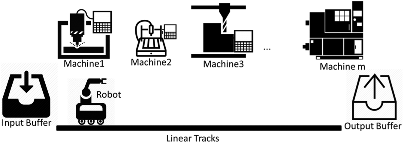
m-machine flexible robotic cell.

Let ε be the loading/unloading time for each machine and each buffer and δ be the robot travel time between the input buffer and the first machine, between two consecutive machines, and between the last machine and the output buffer. d_ab in the following formula gives the certain time needed between the completion times of activities a and b for the robot’s operations such as taking part, moving, and putting the part when activity b follows activity a, that is, d_ab is not related with the process times on the machines

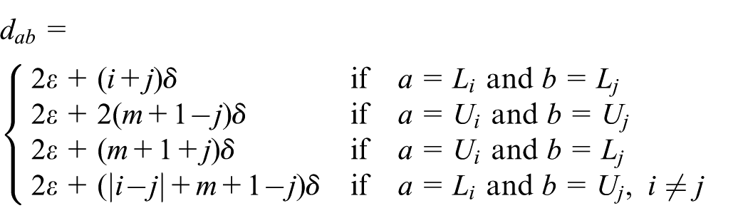
d_{ab} = {\begin{matrix} 2 ε + (i + j) δ & if a = L_{i} and b = L_{j} \\ 2 ε + 2 (m + 1 - j) δ & if a = U_{i} and b = U_{j} \\ 2 ε + (m + 1 + j) δ & if a = U_{i} and b = L_{j} \\ 2 ε + (| i - j | + m + 1 - j) δ & if a = L_{i} and b = U_{j}, i \neq j \end{matrix}

When the process times on the machines are considered, some uncertain amount of waiting time for the robot can be needed. Let’s consider machine i and its loading activity L_i and unloading activity U_i. At the completion time of L_i, the machine starts its operation and finishes it after p time unit. Then, the robot may start unloading this part. During the unloading operation, the robot takes part from machine i (it takes ε time units), moves to the output buffer (it takes $((m + 1 - i) δ)$ time units) and puts the part into the output buffer (it takes ε time units). Thus, the time between the completion of L_i and U_i must be at least $(2 ε + (m + 1 - i) δ + p)$ . There may be several other activities between L_i and U_i, and the total time for performing those activities may not be big enough to complete the process on machine i. In such a case the robot must wait for the end of the process on machine i. The waiting times depend on the order of the activities. Note that d_ab does not contain this uncertain amount of waiting time.

Since the robot performs the same order of activities in a cycle, to prevent permutation and have a fixed cycle, we consider L₁ as the first activity. Thus, the time from L₁ to the next L₁ is the cycle time (T), and the problem is to determine the order of all loading and unloading activities to minimize T. Decision variables

\begin{array}{l} x_{a b} = \\ {\begin{cases} 1 if activity b is performed after activity a by the robot \\ 0 otherwise \end{cases} \end{array}

t_ab: the completion time of activity b when it is performed just after activity a, it is zero if activity b is not performed just after activity a; w_ab: the time that the robot waits before starting activity b when it is performed just after activity a, it is zero if activity b is not performed just after activity a

\begin{matrix} z_{i} = {\begin{matrix} 1 & if L_{i} is performed before U_{i} for machine i \\ 0 & otherwise \end{matrix} \\ min \sum_{a \in A - L_{1}} t_{a L_{1}} \end{matrix}

(1)

\begin{matrix} s . t . \\ \sum_{a \in A - {b}} x_{ab} = 1 \forall b \in A \end{matrix}

(2)

\sum_{b \in A - {a}} x_{ab} = 1 \forall a \in A

(3)

t_{a b} \leq M x_{a b} \forall a \neq b \in A

(4)

w_{ab} \leq p x_{ab} \forall a \neq b \in A

(5)

\sum_{b \in A - {a}} t_{ab} = \sum_{k \in A - {a}} t_{ka} + \sum_{b \in A - {a}} w_{ab} + \sum_{b \in A - {a}} d_{ab} x_{ab} \forall a \in A - L_{1}

(6)

\sum_{a \in A - {L_{1}}} t_{L_{1} a} = \sum_{a \in A - {L_{1}}} w_{L_{1} a} + \sum_{a \in A - {L_{1}}} d_{L_{1} a} x_{L_{1} a}

(7)

\sum_{a \in A - {U_{i}}} t_{a U_{i}} - \sum_{a \in A - {L_{i}}} t_{a L_{i}} \leq M z_{i} i = 2, \dots, m

(8)

\sum_{a \in A - {U_{i}}} t_{a U_{i}} \geq \sum_{a \in A - {L_{i}}} t_{a L_{i}} + (p + 2 ε + (m - i + 1) δ) - M (1 - z_{i}) i = 2, \dots, m

(9)

\sum_{a \in A - {L_{i}}} t_{a L_{i}} \leq \sum_{a \in A - {U_{i}}} t_{a U_{i}} + \sum_{a \in A - {L_{1}}} t_{a L_{1}} - (p + 2 ε + (m - i + 1) δ) (1 - z_{i}) i = 2, \dots, m

(10)

\sum_{a \in A - {U_{1}}} t_{a U_{1}} \geq p + 2 ε + m δ

(11)

t_{ab}, w_{ab} \geq 0 \forall a \neq b \in A

(12)

z_{i} \in {0, 1} z_{i} \in {0, 1}

(13)

x_{ab} \in {0, 1} \forall a \neq b \in A

(14)

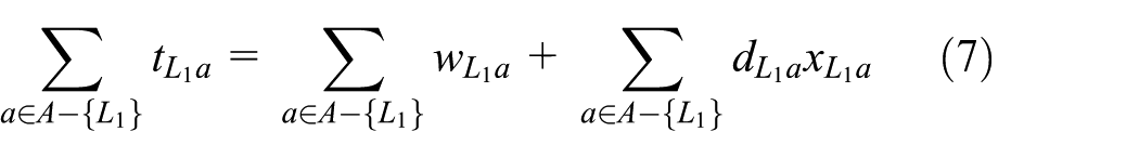
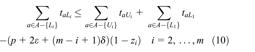
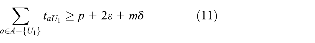
The objective is to minimize the cycle time, which is the time that the robot performs L₁ after the last activity. Note that the cycle starts at the time that L₁ is completed. That time is considered as time zero. During the cycle, all the activities, including L₁, must be completed. So, the end of a cycle is the completion time of L₁, which is also the beginning of the next cycle. By constraints (2) and (3), it is guaranteed that the robot performs all the activities. It passes from one activity to another activity. Constraints (4) and (5) fix t_ab and w_ab variables to zero if the robot does not perform activity b just after activity a. If activity b is performed just after activity a, then x_ab is 1 and the corresponding t_ab and w_ab variables are allowed to be positive by constraints (4) and (5). Note that the waiting time for unloading a part cannot be more than the process time. Because of this in constraint (5), p is used as the coefficient of x_ab instead of a big number M. Constraint (6) is the balance constraint. The completion time of an activity equals to the completion time of the previous activity plus the robot operation times between these two successive activities and plus the waiting time before performing the later activity. Constraint (7) is the balance constraint for L₁. Constraints (8), (9), and (10), together, guaranteed to have enough time between a load of a part and unload of it for finishing its process. Constraint (11) does the same thing for the part processed on the first machine.

The developed SAA

In the attempts of solving the problem using the mathematical models, it is seen that the solution time increases very rapidly when the number of the machines increases, and mathematical model based exact solution methods fails to solve the problems. The SAA is a well-known and efficient meta-heuristic approach. It runs using a single solution at a time, hence does not cause memory shortage problems for even very large-size problem instances. Moreover, it produces a feasible neighboring solution and does not need a repair algorithm, which may lead to highly diversified solutions and deteriorates intensification. Therefore, especially in order to solve large-size problems, an SAA is developed. The method starts with an initial solution which is constructed by any constructive algorithm. At any iteration, the algorithm generates a neighboring candidate solution by making a randomly chosen small change on the current solution. If the candidate solution is better than the current one, the candidate solution is adopted as the new current solution. However, if the candidate solution turns out to be worse than the current solution, the algorithm may either adopt the candidate solution as the next current solution with some acceptance probability or reject it. By giving a chance to move to inferior solutions, the algorithm obtains some capability for escaping from the local minimums. The function that gives an acceptance probability of a bad solution is

EXP (- (F [candidate solution] - F [current solution]) / T)

(15)

where F is the evaluation function, and T is the control parameter of the algorithm called temperature. The probability of accepting an inferior solution decreases if the difference between the current solution and an inferior candidate solution increases, or the temperature drops. At the beginning of the algorithm, the value of temperature is higher, and it falls during the search according to a function known as the cooling schedule that provides intensification over time. Because of the higher value of temperature, initially the algorithm searches the space roughly; however, because of the cooling effect over time, it focuses on some good solution regions. The algorithm stops when a termination criterion is satisfied. Either the number of iterations or the running time or the final value of the control parameter T can be used as the termination criterion. The details of the developed algorithm are given in the following sections.

Representation

A solution is presented by an array having 2m elements in which the numbers of 1 to m correspond to the loading of the first machine to the mth machine, and the numbers of m + 1 to 2m correspond to the unloading of the first machine to the mth machine, respectively. To prevent permutations, the first element of each array is always 1. For example, $L_{1} L_{3} L_{4} U_{2} U_{3} U_{1} U_{4} L_{2}$ order for a four-machine is presented in Figure 2.

Figure 2.

Representation of $L_{1} L_{3} L_{4} U_{2} U_{3} U_{1} U_{4} L_{2}$ order for a four-machine FRC.

Initial solution

After some preliminary experiments and testing different policies, it is decided to generate the initial solutions, randomly. Number 1 is fixed to the first order and then each of the remaining numbers up to 2m assigned to an empty order, randomly. Generating random solutions helps to start from different initial solutions in each run that avoid entrapment in local optima.

Computing cycle time for a given solution

All of the parameters, except waiting times, are easy to compute for finding the objective value of a given solution (an order of the activities). Let’s consider a four-machine case where $ε = 1$ , $δ = 2$ , and p = 80, and the $L_{1} L_{3} L_{4} U_{2} U_{3} U_{1} L_{2} U_{4}$ order for this case. The times needed for performing the robot operations, such as loading, unloading, and transportation, between the successive activities in this order can easily be computed by the d_ab formula. For example, d_L_1L3 is $2 ε + 4 δ = 10$ . Similarly, times between $L_{3} L_{4}$ , $L_{4} U_{2}$ , $U_{2} U_{3}$ , $U_{3} U_{1}$ , $U_{1} L_{2}$ , $L_{2} U_{4}$ , and $U_{4} L_{1}$ are calculated as 16, 12, 10, 18, 16, 8, and 14, respectively.

However, as it is explained in section “The developed SAA,” if the robot turns to a machine for unloading the part earlier than its completion, it should wait. The robot may wait before each of the unloading activities, and these waiting times are not so trivial to compute. Let w_i be the waiting time before performing U_i. Note that these waiting times may be zero. Then, the updated times between the completions of the successive activities in the given order are 10 for L₁L₃, 16 for L₃L₄, (12 + w₂) for L₄U₂, (10 + w₃) for U₂U₃, (18 + w₁) for U₃U₁, 16 for U₁L₂, (8 + w₄) for L₂U₄ and finally 14 for U₄L₁. Thus, the cycle time for this order is $CT = 10 + 16 + 12 + 10 + 18 + 16 + 8 + 14 + w_{1} + w_{2} + w_{3} + w_{4} = 104 + w_{1} + w_{2} + w_{3} + w_{4}$ .

As it is explained in section “The developed SAA,” the time between the completions of L_i and U_i must be at least $(2 ε + (m + 1 - i) δ + p)$ for machine i. When we consider the above-given order, the robot performs the first L₁ and then L₃, L₄, U₂, U₃ and then U₁. Hence, the total time between the completions of L₁ and U₁ is 10 + 16 + (12 + w₂) + (10 + w₃) + (18 + w₁) = 66 + w₁ + w₂ + w₃. This time should be at least $(2 ε + (m + 1 - 1) δ + p) = 90$ . Therefore, on w₁, w₂, and w₃, we have the following condition

66 + w_{1} + w_{2} + w_{3} \geq (2 ε + (m + 1 - 1) δ + p) \Rightarrow w_{1} + w_{2} + w_{3} \geq 24

(16)

When we consider machine 2, U₂ is earlier than L₂ in the given order. So, a part is loaded to machine 2 in a cycle, and it is unloaded in the following cycle. It is shown in Figure 3.

Figure 3.

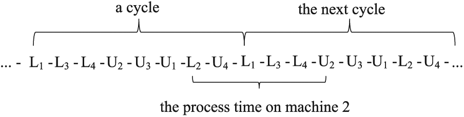
The time from L₂ to U₂ for the order L₁L₃L₄U₂U₃U₁L₂U₄.

The time between L₂ and U₂ is then (8 + w₄) + 14 + 10 + 16 + (12 + w₂) = 60 + w₂ + w₄. This time should be at least $(2 ε + (m + 1 - 2) δ + p) = 88$ . Then, we have the condition

60 + w_{2} + w_{4} \geq (2 ε + (m + 1 - 2) δ + p) \Rightarrow w_{2} + w_{4} \geq 28

(17)

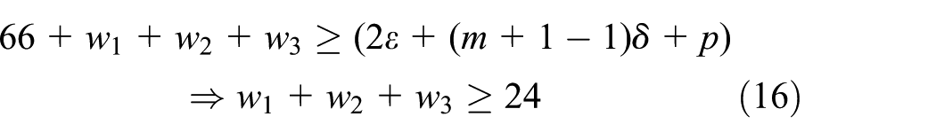
Considering machines 3 and 4, the following conditions are obtained, respectively

38 + w_{2} + w_{3} \geq (2 ε + (m + 1 - 3) δ + p) \Rightarrow w_{2} + w_{3} \geq 48

(18)

64 + w_{1} + w_{2} + w_{3} + w_{4} \geq (2 ε + (m + 1 - 4) δ + p) \Rightarrow w_{1} + w_{2} + w_{3} + w_{4} \geq 20

(19)

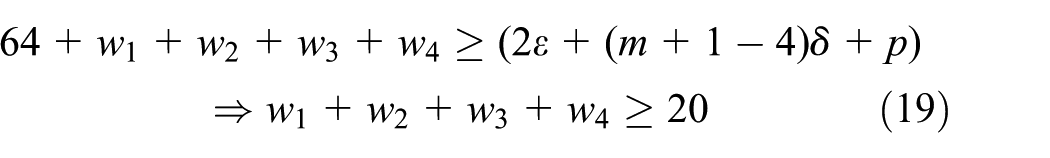
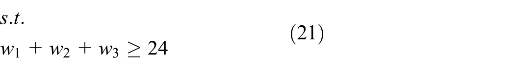
Consequently, the cycle time for the given order is CT = 104 + w₁ + w₂ + w₃ + w₄, and in order to find the minimum CT, the values of w₁, w₂, w₃, and w₄ must be determined considering the above conditions on them. This can be done by solving the following linear programming (LP) model

min CT = 104 + w_{1} + w_{2} + w_{3} + w_{4}

(20)

\begin{matrix} s . t . \\ w_{1} + w_{2} + w_{3} \geq 24 \end{matrix}

(21)

w_{2} + w_{4} \geq 28

(22)

w_{2} + w_{3} \geq 48

(23)

w_{1} + w_{2} + w_{3} + w_{4} \geq 20

(24)

w_{1}, w_{2}, w_{3}, w_{4} \geq 0

(25)

The objective function values of the created orders in the developed SAA are computed by solving such LP models.

Generating candidate solutions

Shift, swap, and reverse operators are used to generate neighboring solutions of the current solution. By the shift operator, the order of a randomly selected activity is changed randomly when the order of the other activities remained the same. Using the swap operator, two activities are chosen randomly, and only their orders are replaced with each other. In the reverse operator similar to the swap operator, two activities are randomly selected. Then, these two activities and all of the activities between these two activities are reversed. Figure 4 gives examples for each of these mechanisms.

Figure 4.

Examples of neighboring solution generating operators: (a) shift operator, (b) swap operator, and (c) reverse operator.

In each iteration of the developed SAA, three new solutions are generated from the current solution using each of the shift, swap, and reverse operators. The objective function of each is computed, and the best of these three new solutions is selected as the generated candidate neighboring solution. This solution is adopted as the next current solution if it is better than the current solution or it is accepted using the acceptance probability function.

Cooling

The geometric cooling, which is the most common cooling method, is applied. According to this method, the developed SAA starts its search at an initial temperature. Then, after each iteration, a certain percent of T is counted as the value of T for the next iteration, that is, T = α*T where 0 < α < 1.

Stopping criterion

A limit on the solution time is used as the stopping criterion. The starting time is kept, and the total time from the starting time to the current time is computed after each iteration. When it exceeds the limit, the search is stopped.

The pseudocode of the developed SAA

The pseudocode of the developed SAA is given below.

Step 0	Set values of the parameters T, Time Limit, α, m, p, ε, and $δ$ . Record the time: Tstart.
Step 1:	Generate the Initial Solution. Current Solution = Initial Solution. Best Solution = Current Solution.
Step 2:	Compute the cycle time of the Current Solution: F[Current Solution]. F[Best Solution] = F[Current Solution]
Step 3:	(a) Generate a neighboring solution of the current solution using the swap mechanism. (b) Generate a neighboring solution of the current solution using the shift mechanism. (c) Generate a neighboring solution of the current solution using the reverse mechanism. (d) Compute the cycle time of these neighboring solutions and select the best of them as the candidate solution.
Step 4:	If F[Candidate Solution] < F[Current Solution] or Rand(0,1) < Exp(-(F[Candidate Solution]-F[Current Solution])/T) then Current Solution = Candidate Solution and F[Current Solution] = F[Candidate Solution]
Step 5:	If F[Current Solution] < F[Best Solution] then Best Solution = Current Solution and F[Best Solution] = F[Current Solution]
Step 6:	Record the current time: Tnow. If the duration from Tstart to Tnow is more than Time Limit, then STOP and present the Best Solution, otherwise T = α*T and go to Step 3.

Experimental results

The performances of the proposed methods are evaluated on several problem instances. In these experiments, an Intel^® Core™ i5-3320 CPU at 2.60 GHz with a RAM of 4.0 GB computer is used for the runs.

Justification of the proposed mathematical model by an exist reference model

The proposed mathematical model is compared with the model presented in Jiang et al.¹¹ Both models have been coded in CPLEX 12.6 software. Table 1 shows the related results, and Figures 5 –7 display the solution times of the models. In the test instances, ε and $δ$ are 1 and 2 time units, respectively.

Table 1.

Results for the mathematical models.

P	Solution times for four-machine FRC (s)			Solution times for five-machine FRC (s)			Solution times for six-machine FRC (s)
P	Optimal cycle time	Referenced model	Proposed	Optimal cycle time	Referenced model	Proposed	Optimal cycle time	Referenced model	Proposed
0	96	1.71	0.09	140	133.32	0.07	192	23,311.81	0.09
25	96	2.43	0.15	140	181.04	0.23	192	240,94.56	0.21
50	96	2.85	0.23	140	101.71	0.21	192	18,434.19	0.29
75	99	1.76	0.59	140	105.16	0.28	192	18,536.08	0.35
100	124	2.18	0.75	140	64.61	4.62	192	9586.02	0.32
125	149	2.01	1.06	153	26.26	31.03	192	5408.44	6.48
150	174	2.53	1.32	178	59.62	34.38	192	4053.00	3.71
175	199	1.90	1.21	203	48.48	40.81	207	2415.22	1635.52
200	224	1.64	1.46	228	39.36	32.98	232	1208.37	506.75
225	249	1.90	1.17	253	33.14	31.47	257	636.32	973.65
250	274	1.70	1.34	278	22.64	35.78	282	1552.92	1231.68

FRC: flexible robotic cell.

Figure 5.

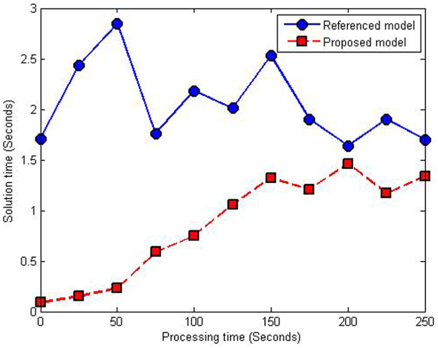
Solution times of the mathematical models for four-machine test instances.

Figure 6.

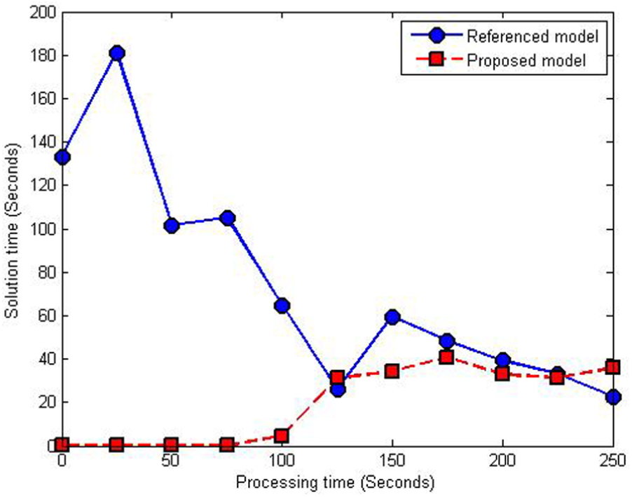
Solution times of the mathematical models for five-machine test instances.

Figure 7.

Solution times of the mathematical models for six-machine test instances.

According to the results in Table 1 and Figures 5 –7, the model proposed in this study solves the problem in a shorter time than the model reported in reference. The solution time of the reference model increases rapidly when the number of the machines increases. The proposed model solves the problem in a concise time when the process time is small. However, much longer times are needed to solve these cases using the other model. Considering higher process times, solution times of the models converge to each other. In these cases, the solution time of the proposed model increases rapidly when the number of the machines increases too. It should be noted that any of the models could not solve problem instances having more than six machines in a cell with high process times.

In Table 1, when the process time is large, the optimal cycle time is larger than the process time by 24; it is larger by 28 in five-machine cell, and by 32 in six-machine cell. By analyzing the robot task sequences derived in experiments, it seems that an optimal cycle time can be derived from a large number of machines. In order to validate or deny this claim 10 instances of FRC problem with four and five machines are solved. In these examples, the process times of the machines are different and randomly selected in [1,100] and [1,300] ranges, where the range of the ε and δ are randomly selected from the [1,4] and [1,5] intervals, respectively. As shown in Table 2, the resulted cycle time indicates that the cyclic times are not harmonic, and it is not predictable from the results of the cell with the fewer machine for a small and large range of process time.

Table 2.

Results of some problems with various process times.

	No.	Four-machine FRC			Five-machine FRC
	No.	P1, P2, P3, P4	ε, δ	Cycle time	P1, P2, P3, P4, P5	ε, δ	Cycle time
Range of P: [1,100]; range of ε and δ: [1,4]	1	12, 80, 81, 96	4, 4	224	12, 80, 81, 96, 42	4, 4	320
	2	9, 94, 67, 47	1, 4	176	9, 94, 67, 47, 35	1, 4	260
	3	62, 64, 92, 48	3, 4	208	62, 64, 92, 48, 8	3, 4	300
	4	5, 19, 60, 61	2, 2	112	5, 19, 60, 61, 92	2, 2	160
	5	69, 10, 51, 7	2, 3	152	69, 10, 51, 7, 22	2, 3	220
	6	11, 16, 49, 95	4, 2	144	11, 16, 49, 95, 87	4, 2	200
	7	64, 11, 28, 39	1, 3	136	64, 11, 28, 39, 68	1, 3	260
	8	7, 52, 25, 63	3, 2	128	7, 52, 25, 63, 76	3, 2	180
	9	38, 95, 80, 100	2, 4	192	38, 95, 80, 100, 38	2, 4	280
	10	69, 71, 97, 85	3, 1	119	69, 71, 97, 85, 83	3, 1	121
Range of P: [1,300]; range of ε and δ: [1,5]	1	135, 114, 190, 142	1, 4	234	135, 114, 190, 142, 83	1, 4	260
	2	225, 46, 191, 103	1, 3	259	225, 46, 191, 103, 78	1, 3	265
	3	165, 37, 43, 199	1, 2	223	165, 37, 43, 199, 115	1, 2	227
	4	131, 111, 176, 187	4, 3	233	131, 111, 176, 187, 293	4, 3	345
	5	296, 42, 180, 258	3, 3	338	296, 42, 180, 258, 35	3, 3	344
	6	116, 194, 250, 137	2, 5	308	116, 194, 250, 137, 246	2, 5	340
	7	19, 247, 81, 278	4, 3	324	19, 247, 81, 278, 33	4, 3	330
	8	37, 211, 97, 242	3, 5	304	37, 211, 97, 242, 172	3, 5	360
	9	87, 137, 45, 298	1, 3	332	87, 137, 45, 298, 251	1, 3	338
	10	40, 281, 247, 45	5, 4	341	40, 281, 247, 45, 213	5, 4	349

FRC: flexible robotic cell.

Performance of the developed SAA

The performance of the proposed SAA depends on the values of its parameters, which are the initial value of T, Time Limit as the stopping criterion, and α. To determine these values, some experiments are needed. Since Taguchi method proposes fractional factorial experiments, it is very effective in parameter setting.³¹ Based on noise minimization, this method selects the best level of the parameters. Using the following equation, the deviation of the response is examined, wherein Y designates the value of reply, and n characterizes the number of orthogonal ranges³²

S / N = {(- 10)}^{*} \log 10 (sum (Y^{2}) / n)

(26)

For each of initial value of T, Time Limit, and α, ranges are determined. These ranges are [90–110] for the initial value of T, [1,5] for Time Limit, and [0.993,0.997] for α. For each of these parameters, three different values are used: (1) the lower bound, (2) the average, and (3) the upper bound of the corresponding range. Thus, nine different combinations of these values are tested. In these tests, the developed SAA is used for solving five different instances which are (4, 75), (6, 150), (8, 250), (10, 500), and (12, 750), where the first entry shows the number of the machines and the second one shows the process time (i.e. (m, p)). For each of the nine combinations of the parameter values, each of these five test instances is solved by the proposed SAA 10 times. The average of the cycle times of the best solutions found by these 10 runs recorded and presented in Table 3.

Table 3.

Computational results for tuning SA parameters.

Combination	SA parameters			Response
Combination	Initial T value	Time Limit	α	(4, 75)	(6, 150)	(8, 250)	(10, 500)	(12, 750)	Sum
1	90	1	0.993	107.2	197.6	325.6	549.6	812.0	1992.0
2	90	3	0.995	107.4	204.8	328.0	550.8	828.4	2019.4
3	90	5	0.997	108.6	197.6	327.2	550.8	806.0	1990.2
4	100	1	0.995	105.6	200.8	324.8	555.6	839.6	2026.4
5	100	3	0.997	107.2	200.8	322.0	557.2	817.2	2004.4
6	100	5	0.993	108.0	205.6	328.0	550.8	815.2	2007.6
7	110	1	0.997	107.6	202.8	326.0	556.0	813.6	2006.0
8	110	3	0.993	107.2	203.6	330.4	553.2	817.2	2011.6
9	110	5	0.995	107.4	202.8	329.6	554.4	828.4	2022.6

SA: simulated annealing.

Then, the S/N ratios are computed using the results in the last column of Table 3. Figure 8 shows the results ofS/N ratios. According to these ratios, when the initial value of T is set to its lower bound (which is 90), Time Limit is set to its upper bound (which is 5 min), and α is set to its upper bound (which is 0.997), the best results are obtained. Thus, these values are used in the following tests.

Figure 8.

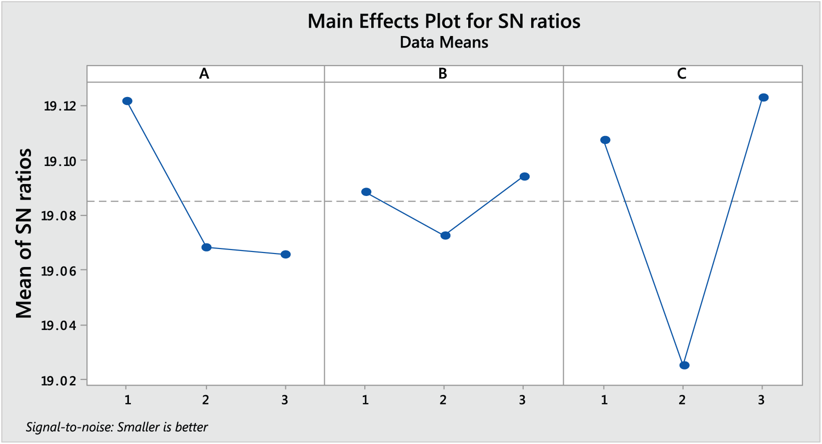
S/N ratio plot for SA parameters.

First, the performance of the proposed SAA is tested on the above test instances whose optimal solutions are found by the mathematical models. Table 4 contains the cycle times and solution times of all the examined test problems for four- to six-machine cells found by the proposed SAA.

Table 4.

Results of the SAA.

P	Four-machine cell			Five-machine cell			Six-machine cell
P	Optimal cycle time	SAA cycle time	SAA solution time	Optimal cycle time	SAA cycle time	SAA solution time	Optimal cycle time	SAA cycle time	SAA solution time
0	96	96	0.033	140	140	0.128	192	192	0.134
25	96	96	0.441	140	140	0.405	192	192	0.321
50	96	96	2.043	140	140	1.260	192	192	0.953
75	99	108.6	2.859	140	140	2.319	192	192	2.215
100	124	124	2.257	140	143.2	4.785	192	192	2.269
125	149	149	1.976	153	160.1	2.741	192	192	4.574
150	174	174	2.049	178	178	2.759	192	197.6	6.203
175	199	199	1.462	203	203	4.087	207	222.7	4.684
200	224	224	2.646	228	228	4.559	232	233	5.778
225	249	249	1.974	253	253	3.344	257	257	5.839
250	274	274	2.536	278	278	4.401	282	282	6.328

SAA: simulated annealing algorithm.

According to the results in Table 4 and Figures 9 –11, the proposed SAA found almost all optimal solutions. Only 6 of the 33 instances could not be solved optimally. In these instances, the gap between the optimal cycle times and the best cycle times found by the proposed SAA is less than 10% of the optimal cycle times. Thus, it may be concluded that the proposed SAA has a very good performance and it may be used to find good solutions to larger instances.

Figure 9.

Solution time of the SAA for four-machine test instances.

Figure 10.

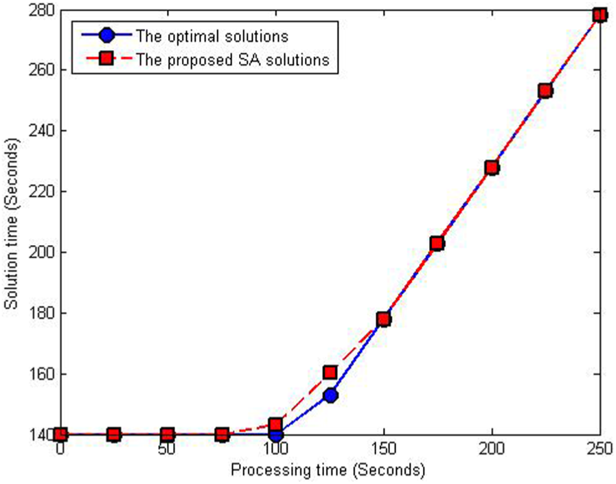
Solution time of the SAA for five-machine test instances.

Figure 11.

Solution time of the SAA for six-machine test instances.

Conclusion

Using TSP’s network flow modeling approach, a novel mathematical model is proposed for solving the cyclic scheduling problem of FRCs with identical and parallel machines which are located on a line. Since the computation time for solving large-sized problems in the model was high, an SAA is examined. The numerical experiments show that the proposed mathematical model performs better in comparison with the one existing in the literature. Solution times by the mathematical models increases very rapidly when the size of the problem increases. The proposed SAA finds almost the optimal solutions of the considered problem instances in affordable short times. This approach might be seen in future studies as a real-time scheduling approach in flexible manufacturing systems. Considering these problems under uncertainty of each parameter can be regarded as another future subject. Finally, it is interesting to consider circular layouts. The cases where machines have buffers with limited capacity may also be considered for future research.

Footnotes

Handling Editor: Chenguang Yang

Declaration of conflicting interests

The author(s) declared no potential conflicts of interest with respect to the research, authorship, and/or publication of this article.

Funding

The author(s) received no financial support for the research, authorship, and/or publication of this article.

References

Barenji

Hashemipour

. A multi-agent RFID-enabled distributed control system for a flexible manufacturing shop. Int J Adv Manuf Tech 2014; 71: 1773–1791.

Ghadiri Nejad

Kovacs

Vizvari

et al . An optimization model for cyclic scheduling problem in flexible manufacturing cells. Int J Adv Manuf Tech 2017, http://doi.org/10.1007/s00170-017-1470-z

Mosallaeipour

Ghadiri Nejad

Shavarani

et al . Mobile robot scheduling for cycle time optimization in flow-shop cells, a case study. Prod Engineer 2017, http://doi.org/10.1007/s11740-017-0784-x

Dawande

Geismar

Sethi

et al . Sequencing and scheduling in robotic cells: recent developments. J Scheduling 2005; 8: 387–426.

Gultekin

Akturk

Karasan

. Scheduling in robotic cells: process flexibility and cell layout. Int J Prod Res 2008; 46: 2105–2121.

Gultekin

Karasan

Akturk

. Pure cycles in flexible robotic cells. Comput Oper Res 2009; 36: 329–343.

Jolai

Foumani

Tavakoli-Moghadam

et al . Cyclic scheduling of a robotic flexible cell with load lock and swap. J Intell Manuf 2012; 23: 1885–1891.

Yildiz

Karasan

Akturk

. An analysis of cyclic scheduling problems in robot centered cells. Comput Oper Res 2012; 39: 1290–1299.

Foumani

Jenab

. Cycle time analysis in reentrant robotic cells with swap ability. Int J Prod Res 2012; 50: 6372–6387.

10.

Foumani

Jenab

. Analysis of flexible robotic cells with improved pure cycle. Int J Comput Integ M 2012; 26: 201–215.

11.

Jiang

Zhang

et al . Single-server parallel-machine scheduling with loading and unloading times. J Comb Optim 2014; 30: 201–213.

12.

Gultekin

Dalgıç

Akturk

. Pure cycles in two-machine dual-gripper robotic cells. Robot Comput Integr Manuf 2017; 48: 121–131.

13.

Foumani

Gunawan

Smith-Miles

. Increasing throughput for a class of two-machine robotic cells served by a multifunction robot. IEEE T Autom Sci Eng 2017; 14: 1150–1159.

14.

Foumani

Smith-Miles

Gunawan

. Scheduling of two-machine robotic rework cells: in-process, post-process and in-line inspection scenarios. Robot Auton Syst 2017; 91: 210–225.

15.

Foumani

Smith-Miles

Gunawan

et al . A framework for stochastic scheduling of two-machine robotic rework cells with in-process inspection system. Comput Ind Eng 2017; 112: 492–502.

16.

Fang

Chen

Liu

. Particle swarm optimization with simulated annealing for TSP. In: Proceedings of the 6th WSEAS international conference on artificial intelligence, knowledge engineering and data bases (AIKED’07), Corfu, 16–19 February 2007. Stevens Point, WI: WSEAS.

17.

Golozari

Jafari

Amiri

. Application of a hybrid simulated annealing-mutation operator to solve fuzzy capacitated location-routing problem. Int J Adv Manuf Tech 2013; 67: 1791–1807.

18.

Golabi

Shavarani

Izbirak

. An edge-based stochastic facility location problem in UAV-supported humanitarian relief logistics: a case study of Tehran earthquake. Nat Hazards 2017; 87: 1545–1565.

19.

Güden

Meral

. An adaptive simulated annealing algorithm-based approach for assembly line balancing and a real-life case study. Int J Adv Manuf Tech 2016; 84: 1539–1559.

20.

Güden

Meral

. An adaptive simulated annealing method for type-one simple assembly line balancing: a real life case study. J Fac Eng Archit Gazi Univ 2013; 28: 897–908.

21.

Prakash

Ceglarek

Tiwari

. Constraint-based simulated annealing (CBSA) approach to solve the disassembly scheduling problem. Int J Adv Manuf Tech 2012; 60: 1125–1137.

22.

La Fata

Passannanti

. A simulated annealing-based approach for the joint optimization of production/inventory and preventive maintenance policies. Int J Adv Manuf Tech 2017; 91: 3899–3909.

23.

Mousavi

Zandieh

Yazdani

. A simulated annealing/local search to minimize the makespan and total tardiness on a hybrid flowshop. Int J Adv Manuf Tech 2013; 64: 369–388.

24.

Abdi

Fathian

Safari

. A novel algorithm based on hybridization of artificial immune system and simulated annealing for clustering problem. Int J Adv Manuf Tech 2012; 60: 723–732.

25.

Leno

Sankar

Ponnambalam

. An elitist strategy genetic algorithm using simulated annealing algorithm as local search for facility layout design. Int J Adv Manuf Tech 2016; 84: 787–799.

26.

Zeb

Khan

et al . Hybridization of simulated annealing with genetic algorithm for cell formation problem. Int J Adv Manuf Tech 2016; 86: 2243–2254.

27.

Naderi

Azab

. An improved model and novel simulated annealing for distributed job shop problems. Int J Adv Manuf Tech 2015; 81: 693–703.

28.

Foumani

Gunawan

Ibrahim

. Scheduling rotationally arranged robotic cells served by a multi-function robot. Int J Prod Res 2014; 52: 4037–4058.

29.

Ghadiri Nejad

Shavarani

Vizvari

et al . Trade-off between process scheduling and production cost in cyclic flexible robotic cells. Int J Adv Manuf Tech 2017; http://dx.doi.org/10.1007/s00170-018-1577-x.

30.

Orman

Williams

. A survey of different integer programming formulations of the travelling salesman problem. In: Optimisation, econometric and financial analysis. Berlin, Heidelberg: Springer, 2007, pp.91–104.

31.

Peace

. Taguchi methods: a hands-on approach. Boston, MA: Addison-Wesley, 1993.

32.

Shavarani

Ghadiri Nejad

Rismanchian

et al . Application of hierarchical facility location problem for optimization of a drone delivery system: a case study of Amazon prime air in the city of San Francisco. Int J Adv Manuf Tech 2017; 1–13, http://doi.org/10.1007/s00170-017-1363-1

A mathematical model and simulated annealing algorithm for solving the cyclic scheduling problem of a flexible robotic cell

Abstract

Keywords

Introduction

Problem definition and formulation

The developed SAA

Representation

Initial solution

Computing cycle time for a given solution

Generating candidate solutions

Cooling

Stopping criterion

The pseudocode of the developed SAA

Experimental results

Justification of the proposed mathematical model by an exist reference model

Performance of the developed SAA

Conclusion

Footnotes

Declaration of conflicting interests

Funding

References