Sage Journals: Discover world-class research

Abstract

We present an anytime-capable fast deterministic greedy algorithm for smoothing piecewise linear paths consisting of connected linear segments. With this method, path points with only a small influence on path geometry (i.e. aligned or nearly aligned points) are successively removed. Due to the removal of less important path points, the computational and memory requirements of the paths are reduced and traversing the path is accelerated. Our algorithm can be used in many different applications, e.g. sweeping, path finding, programming-by-demonstration in a virtual environment, or 6D CNC milling. The algorithm handles points with positional and orientational coordinates of arbitrary dimension.

Keywords

linear paths smoothing merging anytime deviation

1. Introduction

In the area of robotics, the pointwise traversal of a given path is a popular task, e.g. in mobile, industrial or surgical robotics. Describing paths by a sequence of linear segments is the easiest method, and for many tasks the precision of a path approximated by linear segments is sufficient. The movements to be accomplished by a mobile robot or the robot's end-effector are described by a sequence of points in space, that are to be traversed by the robot. In practice, a pre-computed path unfortunately often consists of more path points than are necessary for sufficiently accurate execution. An excessive number of path points renders the movement jerky if the path points are dispersed around the optimal path, leading to unnecessary mechanical stress of both robot and tool. Furthermore, many path points lying close to one another can lead to high computational cost when traversing the path and can reduce traversal speed.

Paths described by teach-in methods are one example where the path can consist of many path points. In this method, the desired movement is recorded while the operator moves the robot's arm, either directly, through a master device or by giving instructions through a control panel. Because of the rather intuitive input of the human operator, the path is subject to deficiencies and frequent unnecessary changes of direction.

The taught-in path can be traversed better after smoothing the path. Another example is voxel-based path planning. Here, only space points with discrete coordinates can be traversed, which may lead to a stair shaped approximation of diagonal lines. Just as with smoothed taught-in paths, smoothed voxel-based paths can be traversed more efficiently, because there are fewer changes of speed and direction, and the total path length is reduced.

The remainder of the text first provides a problem description (Section 2), after which the state of the art is presented (Section 3). Then, the proposed procedure is described in detail (Section 4), and different specializations of the proposed method are shown for points with fixed orientation (Section 5) as well as with variable orientation (Section 6). Finally, experiments are described (Section 7), and open issues and further enhancements are discussed (Section 8).

2. Problem description

The problem of path smoothing can be described as follows. A path P := < p₁, p₂, …, p_n > is given, represented by an ordered list of m-dimensional Cartesian path points p_i := (p_i1, p_i2, … p_im)^T. All path points p_i have the same dimensionality m := m_p + m_o, depending on the degrees of freedom of the robot or the requirements of the task to be performed. The list is sorted in the natural point order, assigning the index 1 to the path's start point and index n to its end point. The parameters m_p, m_o ∈ ℕ, m_p, m_o ≥ 0 designate the dimension of the two coordinate types position and orientation of a path point.

The neighbourhood of a path point p_i is defined as the sequence of points in P between and including the nearest neighbours of that point in the path P to the left and and right of p_i. The deviation d_i between a smoothed path P' and the original path P in the neighbourhood of the path point p_i can be computed according to various error functions, such as the standard deviation or the area spanning both paths. The deviation must be computed differently depending on which coordinate type, position or orientation, is considered.

The error function K represents the criterion used to compute d_i. Its input are the two paths P and P' as well as the index i, and its output is the deviation d_i between them. Finally, we need a threshold value d_lim indicating the maximum allowed d_i. The entire smoothing procedure uses the same K.

If the path points consist of both coordinate types, either position or orientation may, but need not, be used as a constraint. If not only an optimization criterion but also a constraint is being used, a second threshold value c_lim is needed. In that case, we compute a second deviation c_i for each path point which may not exceed c_lim.

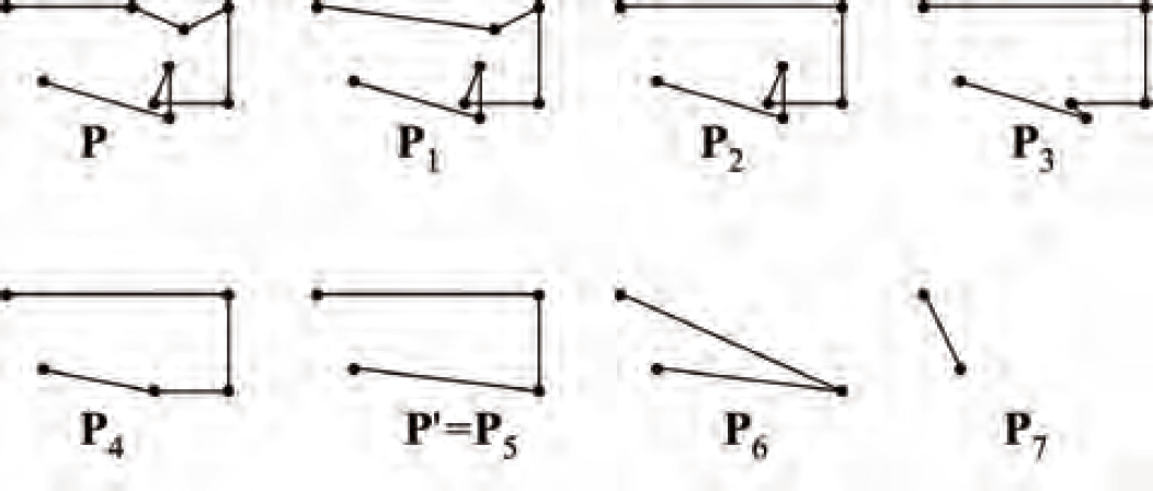
Thus, we search for a path P' whose deviation d_i from P does not exceed d_lim at each individual path point according to K. The number of path points of the path P' is minimized under the given optimization criteria and optionally a constraint (Fig. 1).

Fig. 1.

Example of complete smoothing of a two-dimensional path P with nine path points. In each step i, the path point whose removal leads to the smallest possible deviation between P_i and the original path P is removed, using as criterion the maximum maximum Euclidean distance (see Section 5). A reasonable smoothed path could be e.g. P₅.

3. State of the Art

We can distinguish two main categories of problems where a reduced number of path points is required: path planning and path shortening.

In collision-free motion planning, e.g. for mobile robots, the start and the end points are given, and a path connecting them is sought. There may be obstacles and narrow passages like doors or corridors. A good path avoids all obstacles and is short. In a first step, e.g. using a stochastic approach, in a path planning procedure (Subsection 3.1), a path of possibly poor quality is created, containing many superfluous segments and being much longer than necessary. It is improved in a second step by a path shortening procedure. There is no need for any similarity between the original and the collision-free shortened path apart from having the same start and end point.

In other approaches, the improved path must remain similar to the original path. Not only the start and end point, but also the path between them is provided. However, the quality of this path may be unsatisfying, the path being jerky or consisting of too many segments. In this path smoothing procedure (Subsection 3.2), small deviations from the original path are allowed as long as the number of path segments can be reduced noticably and both paths stay close enough.

3.1 Path planning procedures

In collision-free motion planning, planning is usually performed in the configuration space. The problem of finding a path between a start and an end point is PSPACE-hard in the degrees of freedom and in the number of obstacle surface patches. Therefore, most algorithms in this category are stochastic. Two main classes can be distinguished. Probabilistic roadmap (PRM) approaches (Amato, N.M. & Wu, Y., 1996), (Geraerts, R. & Overmars, M. H., 2002) proceed in two steps. First, a collision-free path is constructed as a graph in robot configuration space. In a second step, pairs of promising vertices are chosen and a simple local planner is used to find a better collision-free connection between them. Approaches based on Rapidly-exploring Random Trees (RRTs) (Kuffner, J. J.; LaValle S. M., 2001), (LaValle, S. M., 1998) use a collision-free path tree that is grown incrementally. In each iteration, a random configuration is chosen, and an attempt is made to find a path to it from the nearest RRT vertex.

Other path planning algorithms exist which do not belong to one of these two categories. One example are potential field based methods which can be used for path planning if there are only few obstacles. One example is the Randomized Path Planner (RPP) (Barraquand, J. & Latombe, J.-C., 1991) where the path is planned according to potential fields and random walks are used to escape from local minima. Another group of path planning algorithms is based on the elastic-band method (Quinlan, S.; Khatib, Q., 1993), where contractive and repulsive forces emanating from obstacles determine the deformation of an original path.

If path segments are to remain piecewise linear, other strategies can be used. Path modifications may be performed by shifting or splitting path segments. Furthermore, path segments can be merged by removing their point of connection (Baginski, B., 1998). A similar procedure is used in (Berchtold, S. & Glavina, B., 1994), where path points are removed based on a heuristic to locally reduce the path length. Another example of collision-free paths for robots can be found in (Urbanczik, C., 2003). Here, path points can be shifted or removed, and segments can be split. After each step the list is resorted by pairs of neighbouring segments. Path smoothing can be performed using a divide-and-conquer algorithm which removes all path points between the first and the last point in one recursion step if the direct path between them is allowed, and otherwise bisects the path points list (Carpin, S.; Pillonetto G., 2006). However, these approaches are not valid for the application we envisage because they do not guarantee a similarity between the original and the smoothed path.

3.2 Path smoothing procedures

In applications where the shortened path must remain similar to the original path, similar strategies can be used, but optimization criteria are different. The simplest form of path smoothing is the removal of superfluous collinear path points, i.e. path points lying on a straight line between their two immediate neighbours. Here, no deviation from the original path arises, but only a few path points can be removed in general. A reduction in the number of path points can also be achieved by approximating the path by curves of a higher degree consisting of nonlinear path segments (e.g., defined by quadratic or cubic functions) (Hein, B., 2003) or non-uniform rational B-Splines (NURBS) (Aleotti, J.; Caselli, S., 2005).

In (Engel, D., 2003) a smoothing procedure for piecewise linear paths is described that removes path points p_j not exceeding a given deviation from a path segment p_i, p_k> with i < j < k. A disadvantage is that the path point list is treated only once and thus some smoothing steps are not executed which are only possible when the path was already smoothed in a previous step.

A well-known point reduction method is linear regression (Bronstein, I. N.; Semendjajew, K. A; Musiol, G.; Mühlig, H., 2001), but it does not guarantee an upper limit for the deviation. Here, a path defined by scattered points is replaced by a path consisting of one straight-line segment placed as close as possible to the scattered points.

3.3 Conclusion

Although a smoothed path slightly deviates from the original path, it can be better suited for a specific application as long as the deviations are not too big.

A downside of the discussed methods is that they are not able to handle paths with both positions and orientations. They are either restricted to one coordinate type (usually positions) or they work in the configuration space. In that space, there is no differentiation into two coordinate types either. Although algorithms working in the configuration space can smooth paths having position and orientation coordinate components, they need a robot model and a forward kinematics.

The path smoothing method we propose offers some advantages which make it particularly suited for time-critical applications working either in configuration space or work space. Due to the order in which the path points are removed, our method has anytime ability, i.e. it can be aborted prematurely and still returns a valid smoothed path, with the result quality increasing monotonically over time. The optimization criterion can be easily exchanged (depending on the application), and an upper bound for the deviation between the original path and the smoothed one can be guaranteed. Furthermore, the algorithm is efficient, as both the computation time and storage space are linear in the number of path points. The algorithm is very versatile due to its capability to handle points with both coordinate types.

4. Path smoothing procedure

The path points p_i are stored in a list ordered by index. Their description (i.e., the Cartesian coordinates) is extended by three components:

The flag r_i ∈ {true, false} indicates whether the path point has been removed while smoothing.

The variable d_i ∈ ℝ indicates the deviation of the path in the neighbourhood of the path point, which will be explained in detail in Section 5. This variable holds the optimization value used to decide which point has to be removed next so that the path deviation stays as small as possible.

The variable c_i ∈ ℝ stores the deviation of the path in the neighbourhood of the path point according to a second coordinate type. This variable holds the constraint value. The use of c_i is detailed in Section 6. If the path has only one coordinate type, c_i is not used ¹.

The path points removed during path smoothing are not deleted from the list, but are instead only marked as removed, since the procedure must be able to access the original path at any time. When smoothing is complete, all path points not marked as removed are copied into a target path point list containing only the path points of the smoothed path.

The algorithm for removing path points works as follows:

For all path points p_i, set r_i = false and c_i = 0.

For all path points p_k not yet removed (r_k = false), compute the arising deviation d_k between the smoothed path P' and the original path P, assuming that p_k is removed from the path (in addition to the path points removed so far). If a constraint is being used, compute c_k.

Select among all path points with c_k < c_lim the path point p_k with the smallest d_k.

3a
If the deviation d_k is smaller than the specified value d_lim, then mark p_k as removed (r_k = true) and go to (2).
3b
Otherwise, no further path points can be removed from the path, and the path P' := < p_i | r_i = false >, i = 1, …, n is returned.

If no constraints are being used, no computations of c_i are performed and c_i stays zero, being without any effect.

The path point whose elimination leads to the smallest deviation from the original path while not violating the constraints is removed during each iteration. In this way, it is ensured that a (locally) maximum number of path points can be removed before the deviation locally exceeds the threshold d_lim and the algorithm terminates.

In order to prevent gradual drifting of the path in each iteration, the current path must not be compared with the path from the previous iteration step, but with the original path.

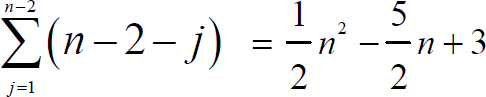
A certain computational speed improvement can be obtained by using an efficient implementation. Given a path with n path points, the maximum smoothing of the path would require n-2 iterations, as the first and last path point are not removed. For a given iteration step j, the number of local deviation computations is n-2 - j. This belongs to the complexity class O(n²), since the total number of computation steps is
$\sum_{j = 1}^{n - 2} (n - 2 - j) = \frac{1}{2} n^{2} - \frac{5}{2} n + 3$
(1)

The procedure can be accelerated by considering that the path deviation only changes in the neighbourhood of a path point that is removed. For this purpose, the component d_i of all path points p_i is required to buffer the corresponding deviation.

After a path point has been removed, the deviation can change only for the two neighbouring path points. Therefore, only two instead of n-2 - j deviations need to be determined per iteration step. This results in a complexity of
$n + \sum_{j = 2}^{n - 2} 2 = n + 2 (n - 3) = 3 n - 6$
(2)

computation steps, with complexity dropping from O (n²) to O (n). The same holds true for the computation of the constraint c_i, which, if used, is computed whenever d_i is computed.

In the following, we describe how the interval of path points needed for the computation of the deviation d_i is determined. We are looking for two path points p_min and p_max that border on the interval in question: I := [p_min; p_max] = < p_min, …, p_i, …, p_max>.

In the first iteration no path points have been removed yet. Trivially, only three path points need to be regarded: the path point p_i as well as its neighbours p_i-1 and p_i+1, and the path segment < p_i-1, p_i, p_i+1 > must be compared with < p_i-1, p_i+1 > to compute d_i. The manner in which this comparison is performed depends on the error function used and is described in Section 5.

In the subsequent iterations we must consider which path points are removed and must extend the path interval of interest beyond the previously removed path points so that its borders again consist of the next two non-removed path points p_min and p_max. Thus p_min and p_max are the direct neighbours of pi that have not yet been removed. The deviation d_i is computed by comparing a path segment of the original path P_i,o = [p_min, p_max] = < p_min, …, p_i, …, p_max > and the corresponding path segment on the smoothed path P_i,t = < p_min, p_max>.
5. Path deviation functions for a fixed orientation

In this section, we consider only paths with positional coordinates and no orientation and we do not use any constraints (Waringo, M.; Henrich D., 2006). Depending on the application, different error functions K can be used. We investigated three error functions:

• K₁: d_i is the maximum Euclidean distance between the smoothed path from the original path in the interval P_i,o. This criterion can be used in applications where motion is constrained to a safety corridor, e.g. in a master-slave robotic guidance system, car manufacturing, or robotic endoscope holding systems.

K₂: d_i is the root-mean-square deviation of the path points in the original path P_i,o from the smoothed path P_i,t in the interval P_i,o. This is the square root of the mean of the squares of the shortest distances between each of the path points p_i ∈ P_i,o and the segment P_i,t. This criterion is useful mainly for theoretical analysis.

K₃: d_i is the area between the smoothed paths segment P_i,t and the corresponding segment P_io on the original path. K₃ is the best choice for sweeping applications, e.g. bones milling or cleaning robots.

The first two error functions can be determined quickly and work for path points with any dimensionality. Error function K₃ is useful and intuitively plausible for paths defined in a plane, i.e. two-dimensional paths. However, K₃ can also be used for more dimensions.

The error function K₁ guarantees that the smoothed path never deviates by more than the distance d_lim from the original path. One disadvantage involves the computation of each deviation d_i: Only one path point p_i ∈ [p_min; p_max] is used and the distance from the other path points in that interval is neglected. Path points far away from P_i,t are rated strongly, whereas a constant slight deviation of the path across all path segments under consideration leads to a smaller deviation.

This drawback can be avoided by using the error function K₂ as this function uses all path points p_i ∈ [p_min; p_max] for the computation. Nevertheless, path points far away from P_i,t are recognized because the distance to the smoothed path P_i,t is squared. The computation of K₂ is also quite fast.

The computation of K₃ is more costly, however unlike K₁ and K₂ it also considers the distance between the individual path points p_i ∈ [p_min; p_max], not just in relation to P_i,t.

Fig. 2 illustrates the three error functions.

Fig. 2.

Sketch describing the determination of path deviation d_i. The linear path segments to be compared are the original path (a) and the smoothed path (b). The error functions K₁, K₂, and K₃ are illustrated in (c), (d), and (e)

The algorithm uses the heuristic of always removing the point yielding the smallest deviation. Although this provides good results in practice, the path obtained is not necessarily globally optimal. Because the algorithm does not look ahead to try to remove more than one path point at a time and does not allow the deviation to exceed the limit d_lim in any iteration step, opportunities to shorten the path can be missed. Consider for example Fig. 3 (a). When using criterion K₁ and a maximum allowed deviation d_lim = 0.5 ⋅ ‖ p₂ p₃ ‖ (half the distance between p₂ and p₃), the optimal path (b) cannot be obtained. The removal of either p₂ or p₃ leads to a deviation that is too high. The smoothing procedure aborts without being able to remove p₂ and p₃.

Fig. 3.

Example for the non-optimality of the proposed algorithm. (a) A path consisting of five points, (b) the optimal path with a maximum allowed deviation of 0.5 ⋅ ‖ p₂ p₃ ‖

Nevertheless, the paths created are valid because the deviation does not exceed the maximum allowed. An advantage of the proposed method is that the algorithm is anytime capable, i.e. it can be aborted prematurely and still delivers a valid result. The quality of the path increases monotonically until termination. This is an important feature for time-critical applications, such as sensor-based motion planning.

6. Path deviation functions for variable orientations

In Section 5 paths with arbitrary dimensionality, but just one coordinate type have been treated. However, Cartesian paths whose points contain information on both coordinate types (position as well as orientation) cannot be handled reasonably with this approach, as positions and orientations can not be treated in the same way. For example, a positional value is unrestricted, whereas an orientation is restricted to the angle range [–180°, +180°].

Therefore, we choose to compute position and orientation separately and combine positional and orientational deviation in an optimization procedure as optimization criterion and/or constraint, respectively. At that point, both are real numbers which are compatible again.

We use quaternions for representing the orientation of a path point, we decided to use the representation in (Maillot, P., 1990). This representation overcomes severe disadvantages of a vector angle representation like e.g. Euler angles.

Eq. (3) shows the representation of an orientation o_i = φ i as a quaternion.

q_{i} = a_{i} + b_{i} \cdot j + c_{i} \cdot k + d_{i} \cdot l w i t h a_{i}, b_{i}, c_{i}, d_{i} \in R .

(3)

Just like the distance between two positions can be computed, we can easily obtain the distance between two orientations, it corresponds to the angle between the orientations:

d_{p} (p_{1}, p_{2}) = \sqrt{(p_{2, x} - p_{1, x})^{2} + (p_{2, y} - p_{1, y})^{2} + (p_{2, z} - p_{1, z})^{2}}

(4)

d_{o} (O 1, O 2) = a c o s (a_{1} \cdot a_{2} + b_{1} \cdot b_{2} + c_{1} \cdot c_{2} + d_{1} \cdot d_{2})

(5)

From Eq. (4), it is obvious that the distance between two orientations can not exceed the range [–180°, +180°] whereas the distance between two points is unrestricted, Eq. (5).

The criteria K₁ and K₂ are directly applicable for orientations if we replace Eq. (4) by Eq. (5) in the computation. For criterion K₃, we need to obtain the cumulated orientational deviation. We solve that problem by numerically integrating the orientational deviation along the path between two path points. We need to interpolate orientations. Quaternion interpolation can be performed using either lerp or slerp interpolation (Maillot, P., 1990). Although slerp interpolation is slightly more computationally expensive, we chose to use slerp as lerp interpolation yields only an approximated result.

Slerp interpolation works as follows. Let p = 1, … 0 be a control parameter, q₁ and q₂ two orientations given as quaternions and the angle θ between q₁ and q₂, as computed in Eq. (6), (7) and (8).

We obtain the control variables

r_{1} = s i n ((1 - p) \cdot θ) / s i n (θ)

(6)

r_{2} = s i n (p \cdot θ) / s i n (θ)

(7)

and the slerp-interpolated orientation

q^{'} = r_{1} \cdot q_{1} + r_{2} \cdot q_{2} \cdot

(8)

By summing the orientational deviations of a smoothed path segment from the corresponding unsmoothed segment, we obtain the orientational deviation using criterion K₃. For this, we do not directly use the unsmoothed path, but the segmentwise projection of the unsmoothed path onto the smoothed path. To illustrate this idea, we show the interpolation of the orientation for the orientational dimensionality mo = 1 and the obtained deviations as well as the sum of the deviation (Fig. 4).

Fig. 4.

Sketch visualizing the computation of the angle sum Δφ. For simplification, the angle is represented only in 1D. Top: Curve progression of the orientation of a smoothed path [p_min, p_max] (blue) and the original path [p_min, …, p_i-1, p_i, p_i+1, …, p_max] (red). Bottom: Curve progression of the angle deviation q between the two paths

For m_o = 2 or m_o = 3, the procedure works in exactly the same way, as Eq. (5) and Eq. (8) are handling 3D orientations. Orientations of higher dimensionality, although untypical in practical applications, can also be easily used if the path deviation functions are adapted accordingly, just like positions of higher dimensionality are usable.

In a simple optimization procedure, the computed positional and orientational deviations p_i and o_i are assigned to the optimization and constraint value c_i and d_i. If not both coordinate types are used, all c_i stay zero and the algorithm works without any constraint. On the other hand, the optimization value d_i is indispensable. We obtain five different cases, as shown in Table 1.

Table 1.

Enumeration of the five possible cases when combining both coordinate types. The table entries indicate the assignments of the path points' positional and orientational deviation p_i and o_i to the algorithm's values c_i and d_i, as well as the assignments of the indicated positional and orientational deviation limit values p_lim and o_lim to the algorithm's values c_lim and d_lim.

	Case
	(a)	(b)	(c)	(d)	(e)
Optimization value d_i	p _i	o _i	p _i	o _i	p_i/p_max + o_i/o_max
Max. optimizat. deviation d_lim	p _lim	o _lim	p _lim	o _lim	2
Constraint value c_i	/	/	o _i	pi	/
Max. constraint deviation c_lim	/	/	o _lim	p _lim	/

Case (a) is the case seen in Section 5. No orientational information is evaluated, and there is no constraint. The computed positional deviation p_i is used as d_i in the path smoothing procedure. Similarly, in Case (b), we are smoothing orientations without using constraints. The criterion function used to compute d_i is the version adapted to orientations (Eq. (5)), and the deviation d_i used in the optimization procedure is the orientational deviation o_i.

In Case (c), the positional deviation is used as in (a) as optimization value, but in addition we use the orientation as constraint. As long as the limit is not exceeded (c_i < c_lim) in any point with the lowest positional deviation, the path is smoothed as in Case (a). Points whose orientational deviation o_i exceed o_lim are not removed, no matter how low p_i is. Case (d) is analogue to Case (c), the roles of position and orientation being exchanged.

In Case (e), we have to optimize the position and orientation simultaneously. Because they are incompatible, we have to use a little trick. We normalize p_i and o_i to p_lim resp. o_lim, giving an indication on how close both deviations are to the limit and bringing them into the same domain. Now, we can simply sum up both values to obtain d_i. The ratio between p_lim and o_lim correlates linearly with the relation of the influences of position and orientation. As both p_i / p_max and o_i / o_max are positive numbers and their sum may not exceed 2, both positional and orientational deviations are restricted to twice the maximum indicated.

7. Experiments and Results

In this section, we present and analyze a practical surgical application of our algorithm. First, we compare the results yielded when applying the three error functions described previously. Then, we briefly describe the original paths used in the surgical application and their drawbacks. Finally, we describe the improvement achieved by applying the smoothing algorithm.

In the first rather theoretic experiment, a perturbed linear path consisting of 1000 points, positioned equidistantly on the x axis in the interval [0; 1000] with increasing x coordinate and distributed uniformly on the y axis with y values between −10 and +10, is smoothed using criterion K₁ (maximum deviation). The y coordinate of the first and the last point is 0.

Fig. 5 shows the results of the path smoothing.

Fig. 5.

Remaining path points, path length and maximum deviation against computation time T [ms] for a perturbed linear path segment

This experiment demonstrates the nice anytime property of the algorithm. It can be aborted at any moment. With a maximum deviation of only 1 mm, reached after 20 ms, already one third of the path points could be removed. The correlation of computation time and number of path points removed is nearly linear. After less than half of the time needed for complete smoothing, half of the path points have been removed.

However, this experiment also shows the non-optimality of the algorithm. Because the first and the last point have a y coordinate of 0 and the y coordinate of all other points lies in the interval [-10; 10], the path could be reduced to its start and end point with a maximum deviation d_lim =10 mm. Yet, in general the algorithm finds that solution only at d_lim = 20 mm.

When milling cavities in workpieces, problems with overly fragmented and angulated milling paths arise, cf. the RONAF project (Robot-based Navigation for Milling at the Lateral Skull Base (Federspil, P. A.; Geisthoff, U. W.; Henrich, D. & Plinkert, P. K., 2003)) (Fig. 6). The goal of the RONAF project is the development and examination of a system for navigation on the lateral skull base with the purpose of an interactive supervision of a surgical robot during interventions. Modular navigation and control procedures are being used. The operation is planned on a preoperatively acquired 3D dataset, e.g. computed tomography (CT) or magnetic resonance tomography (MRT). The robot and its attached tool are moved relative to this dataset. Milling in the skull bone demands extreme precision (with tolerances well below one millimeter) in spite of the high force required to remove larger quantities of bone, a combination that is very straining for a surgeon and poses little problem to a robot. Therefore an important increase of processing quality can be expected.

Fig. 6.

Experimental setup from the RONAF project.

In the RONAF system, three-dimensional path planning (Waringo, M.; Henrich D., 2004) is used in order to mill out a given implant volume with a robot-controlled miller. The paths planned in a voxel space are angled and are often represented by an excessive number of path points. The robot follows the path points by interpolating linearly between two successive path points. By reducing the number of path points, we can significantly reduce the milling duration.

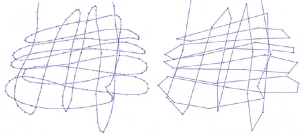
Path smoothing was applied to milling paths planned in a voxel space for milling a hearing aid implant volume (Fig. 7). The milling time for the non-smoothed path is unsatisfactory long. The traversal speed is strongly reduced in regions where the path points are close to each other or where the directional change between two consecutive path segments is high. This drawback is due to robot dynamics restrictions such as the maximum acceleration in the robot joints and restrictions involving computing time (i.e. the maximum number of path segments that can be processed per second).

Fig. 7.

Milling paths for the hearing aid implant Vibrant Soundbridge (Siemens/Symphonix). The circular paths lie is the horizontal plane, and path segments perpendicular to that plane are vertical segments. Upper left: original path planned in a voxel space, upper right: close-up of the original path (4403 path points), bottom left: path with maximum deviation of 0.18 mm (2788 path points), lower right: path with maximum deviation of 0.35 mm (1405 path points)

Part of the robot motions occurs above the workpiece (the long straight segments in Fig. 7), where the tool moves above the bone without touching it. These segments serve to change the currently processed region. These path segments cannot be removed, since otherwise the miller would mill bone at invalid locations. The path smoothing only applies to the horizontal path segments located in the bone. The smoothing algorithm was applied to the entire path, with all vertical and horizontal path segments needed for changing a region marked as non-removable. While keeping the modification to the path at a non-critical level so that noticeable changes occur in the milled geometry ², the number of path points can be reduced by more than 50%, as shown in Table 2. With an acceptable tolerance of 0.35 mm, it is possible to eliminate about 46% of the milling duration, 69% of the path points and 65% of all directional changes normally arising in the non-smoothed path. The computation time for path smoothing was measured on an AMD Athlon XP 2600+ PC with 512 MB of RAM. The computation time is nearly exactly linear with the number of points removed, in this example about 0.6 ms per point.

Table 2.

Number of path points remaining, necessary time requirement for traversal and for path smoothing, path length and angular integral in the function of the maximum allowed deviation.

maximum deviation d_lim [mm]	# path points	time req. for path traversal [min:sec]	comp. time [sec]	path length [mm]	angular integral [°]
0	4403	12:35	0.00	5545	239,417
0,10	4355	12:24	0.05	5527	234,048
0,13	2788	09:22	0.94	5460	150,501
0,18	2107	08:06	1.32	5427	118,268
0,25	1629	07:12	1.58	5403	96,645
0,35	1405	06:44	1.77	5367	82,650
0,60	1207	06:19	1.80	5334	74,520
1,00	1098	06:05	1.88	5306	72,273
2,00	997	05:49	1.90	5232	69,016
Infinite	832	04:21	2.04	4171	58,320

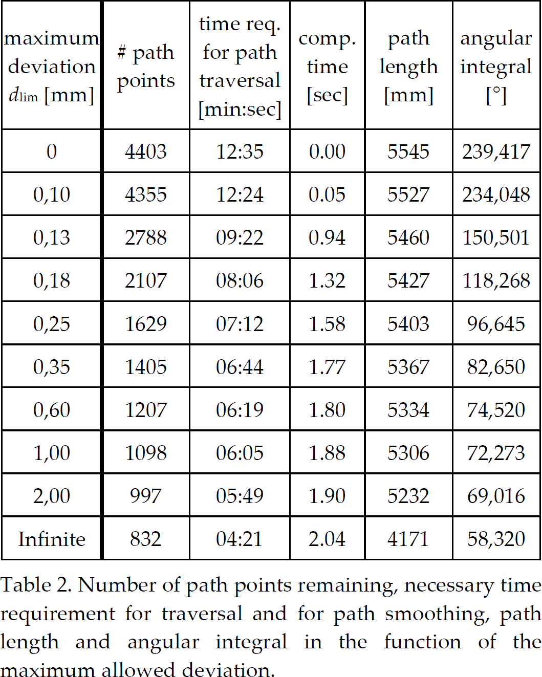
Table 3 shows a comparison of paths smoothed using the three error functions and evaluated according to the three error functions. As expected, path planned with error function K_i, i ∈> {1,2,3} ranked best when the evaluation was performed according to the same error function K_i. No clear advantage can be determined and no error function is made redundant by the other two.

Table 3.

Comparison of the three error functions K₁, K₂ and K₃ when reducing the milling path of the implant Vibrant Soundbridge from 4403 to 1500 path points. K₁: maximum deviation, K₂: root-mean-square deviation, K₃: spanned area. The error function used for path planning is noted in the rows and the error function used for evaluation is noted in the columns. In the cells, the deviations are noted, with both the maximum and the average value per path segment.

		Error function for path evaluation
		K₁ [mm]	K₂[mm²]	K₃[mm²]
Error function for path computation	K ₁	max : 0,281	max: 0,078	max: 2,125
	K ₁	avg: 0,171	avg: 0,015	avg: 0,257
	K₂	max: 0,478	max: 0,046	max: 1,531
	K₂	avg: 0,216	avg: 0,019	avg: 0,358
	K₃	max: 0,884	max; 0,297	max: 0,393
	K₃	avg: 0,197	avg: 0,020	avg: 0,213

Another example of path smoothing in the RONAF project is shown in

Fig. 8. In order to record an ultrasound image of the patient's skull, the skull is sampled manually with the tip of an infrared marker whose spatial position is sampled at equidistant times. This path is then traversed by the robot, an ultrasound head being mounted on the effector. Between recording and traversing of the path, smoothing is performed. This way, in addition to rendering the path less jerky, there are also agglomerations of path points being removed which appear when the surgeon interrupts the movement of the marker.

Fig. 8.

Scanline path for ultrasound recording of the human skull. Left: original path (307 path points), right: smoothed path using K₁ and d_lim = 1 mm (90 path points).

8. Conclusions

We have presented a method that smooths paths of any dimensionality consisting of linear segments until the deviation between the smoothed path and the original path locally exceeds a given threshold. The error function for deviation determination can easily be exchanged and adapted for diverse applications. By introducing the additional variables d_i and c_i and flag r_i for each path point, the computational requirement is reduced from quadratic to linear in the number of path points used.

Our method is anytime-capable, i.e. it can be aborted at any moment and returns a valid resulting path for which the maximum deviation increases monotonically and the number of path points decreases monotonically in the allowed computation time. There is no need for an additional increase in computation speed and the storage requirement is also not critical, as it is linear with respect to the number of path points.

Possible extensions of the algorithm include the consideration of forbidden regions that may not be crossed by the path and a distance computation that varies depending upon the position on the path.

If applied to motion planning in a cluttered environment, the algorithm does not handle collisions with obstacles close to the unsmoothed path. In this case, further conditions are required which are evaluated in addition to the error functions and which avoid the smoothed path getting too close to the obstacles. In this scenario, the geometry of the actuator must be considered too.

For a path smoothing with using both positions and orientations as optimization criterion (Case (e) in Section 7), one could in addition use one of them as constraint, giving even more control over the maximum allowed deviation.

If a globally optimal path has to be found, the presented method is not suitable, as it is a local method and can get stuck in local optima, as shown in the first experiment. In order to overcome this disadvantage, a global method has to be used.

Footnotes

9.

This work has been supported by the German Research Foundation (DFG) under the project name “Robotergestützte Navigation zum Fräsen an der lateralen Schädelbasis” (RONAF) with the identifier 227100. Further information can be found at http://ai3.inf.uni-bayreuth.de/projects/ronaf .

1

This is realised by initially setting cⁱ = 0 and not modifying it any more and setting clim to an arbitrary value >0.

2

As the miller's diameter is 4.5 mm and the robot's repeatability accuracy is 0.35 mm, a maximum deviation in the path of 0.35 mm is deemed acceptable.

References

Aleotti

Caselli

(2005). Trajectory clustering and stochastic approximation for robot programming by demonstration, pp. 2581–2586, IEEE/RSJ Int. Conf. On Intelligent Robots and Systems

Amato

N.M.

& Wu

(1996). A randomized roadmap method for path and manipulation planning, Proceedings of the IEEE Int. Conf. Robot. & Autom., pp. 113–120.

Baginski

(1998). Motion planning for Manipulators with Many Degrees of Freedom – The BB Method, Doktorarbeit, TU München

Barraquand

& Latombe

J.-C.

(1991). Robot motion planning: a distributed representation approach, Int. Journal of Robotics Research, 10 (6), pp. 628–649, 1991

Berchtold

& Glavina

(1994). Kosten-Nutzen-optimale Verbesserung kollisionsfreier Roboterbewegungen mittels Polygon-Manipulation, in: 10. Fachgespräch Autonome mobile Systeme

Bronstein

I. N.

Semendjajew

K. A.

Musiol

Mühlig

(2001). Taschenbuch der Mathematik, Verlag Harri Deutsch, ISBN 3-8171-2005-2

Carpin

Pillonetto

(2006). Motion planning using adaptive random walks, IEEE Transactions on Robotics and Automation, 21 (1)

Engel

(2003). Sensorgestützte Robotersteuerung für den Einsatz in der Chirurgie, Dissertation, Fakultät für Informatik der Universität Fridericiana zu Karlsruhe (TH)

Federspil

P. A.

Geisthoff

U. W.

Henrich

& Plinkert

P. K.

(2003). Development of the First Force-Controlled Robot for Otoneurosurgery, Laryngoscope 113:

10.

Geraerts

& Overmars

M. H.

(2002). A comparative study of probabilistic roadmap planners. In Proc. Int. Workshop on Algorithmic Foundations of Robotics (WAFR),

11.

Hein

(2003). Automatische offline Programmierung von Industrierobotern in der virtuellen Welt, Dissertation, Fakultät für Informatik der Universität Fridericiana zu Karlsruhe (TH), 2003.

12.

Kuffner

J. J.

LaValle

S. M.

(2001). RRT-Connect: An efficient approach to single-query path planning, in Proceedings of the IEEE Conference on Robotics and Automation, San Francisco, pp. 995–1001.

13.

Maillot

(1990). Using quaternions for coding 3d transformations, in Graphics Gems I, Academic Press Inc., Boston pp. 498–515

14.

Quinlan

Khatib

(1993). Elastic bands: Connecting Path Planning and Control, in Proceedings of the IEEE Conference on Robotics and Automation, Atlanta, pp. 802–807.

15.

LaValle

S. M.

(1998). Rapidly-exploring random trees: A new tool for path planning, TR 98–11, Computer Science Dept., Iowa State University

16.

Urbanczik

(2003). SIMERO: Bildbasierte Kollisionserkennung und Bahnglättung im Konfigurationsraum, diploma thesis, Fakultät für Informatik, Universität Kaiserslautern, D-67653 Kaiserslautern

17.

Waringo

Henrich

(2004). 3-Dimensionale schichtweise Bahnplanung für Any-Time-Fräsanwendungen, Robotik, München/Germany

18.

Waringo

Henrich

(2006). Efficient smoothing of piecewise linear paths with minimal deviation, Proceedings of the IEEE/RSJ International Conference on Intelligent Robots and Systems, Beijing/China, pp. 3867–3872

Smoothing of Piecewise Linear Paths

Abstract

Keywords

1. Introduction

2. Problem description

3.1 Path planning procedures

3.2 Path smoothing procedures

3.3 Conclusion

4. Path smoothing procedure

Footnotes

9.

1

2

References