Experimental Validation of a Dynamic Model for Lightweight Robots

Abstract

Nowadays, one of the main topics in robotics research is dynamic performance improvement by means of a lightening of the overall system structure.

The effective motion and control of these lightweight robotic systems occurs with the use of suitable motion planning and control process. In order to do so, model-based approaches can be adopted by exploiting accurate dynamic models that take into account the inertial and elastic terms that are usually neglected in a heavy rigid link configuration.

In this paper, an effective method for modelling spatial lightweight industrial robots based on an Equivalent Rigid Link System approach is considered from an experimental validation perspective.

A dynamic simulator implementing the formulation is used and an experimental test-bench is set-up. Experimental tests are carried out with a benchmark L-shape mechanism.

1. Introduction

Nowadays, one of the main topics in robotic research is dynamic performance improvement. In order to achieve this, the goal is to increase the working velocity and lighten the structure while maintaining a high degree of precision and accuracy. Some successful examples of this direction are the well-known closed-loop robots Delta robot, e.g., ABB Flex-Picker [1], and the ELAU Robot D2 [2].

In this framework, if the links are lightened and made slender, inertial and elastic effects have to be carefully evaluated, taken into account and controlled for since they can cause vibrations, lack of precision, premature wear, mechanical breaking and control instability.

Different approaches can be adopted to limit or turn down such effects, starting from ad-hoc non model-based trajectory planning techniques [3,4]. Indeed, it is essential that motion laws induce forces and torques at the joints compatible with the given constraints, thereby reducing the possibility of exciting mechanical resonance modes that are most often not modelled. This means that the planning algorithms output has to be a smooth trajectory, i.e., a trajectory with a high order of continuity, at least ensuring the continuity of the joints' acceleration to obtain trajectories with a limited jerk. As demonstrated in [5,6], limiting the jerk reduces the wear of the robotic system and reduces the excitation of resonant frequencies.

In recent works, hybrid time-jerk optimal trajectories and a high degree of continuity trajectories have been proposed [5–15], in order to take advantage of jerk reduction while planning fast trajectories.

On the other hand, if the model of the robot is considered in the motion planning and control, lightening the structure and increasing the working velocity do not allow for the adoption of the hypothesis of link/arm rigidity. Thus, effective dynamic models that include inertial and elastic effects have to be set-up. Some effective examples of model-based control of lightweight mechanisms can be found in [16–20].

Many dynamic models have been proposed in the existing literature for multibody rigid flexible-link robotic systems. However, this topic is still open to investigation - in particular, if spatial systems, such as the common industrial robot configurations, are considered or experimental and non-numerical validation is addressed [22–24].

In this attempt, a first experimental validation of a dynamic formulation for lightweight robots is carried out.

In Section 2, the dynamic model is summarized, while in Section 3 a first experimental validation is presented and the results discussed.

2. ERLS-FEM model

The method under validation, based on an Equivalent Rigid Link System (ERLS) concept [24], is intended for use in the accurate dynamic modelling of robotic systems with large displacements and small elastic deformation. This covers the working conditions of a classical industrial robot, e.g., an anthropomorphic robot, with light and slender links. The approach, here called ERLS-FEM and presented in [25-26], basically defines the elastic displacements with respect to an Equivalent Rigid Link Mechanism (ERLS) and each link is evaluated by means of spatial beam finite elements (FEM). In this approach, the kinematic equations of the ERLS are decoupled from the compatibility equations of the displacements at the joints, the mutual influence between gross body motion and vibration is taken into account and 3D kinematics formulations such as the Denavit-Hartenberg (D-H) notation can be adopted to formulate and solve the ERLS kinematics. The results can then be used and easily integrated in the equations of the dynamic model of the flexible multibody system.

One of the main features of the method is that it allows the use of standard frame and kinematic notations, thus simplifying the roboticist approach to the method.

2.1. Kinematics

Being {X, Y, Z} a fixed global reference frame, let ui and ri be the vector of the nodal elastic displacements of the i-th finite element and the vector of the nodal position and orientation for the i-th element of the ERLS respectively, and wi and vi be the position vector of the generic point of the i-th element of the ERLS and its elastic displacement respectively, the absolute nodal position and orientation of i-th finite element bi with respect to the global reference frame is:

${\mathrm{b}}_{\mathrm{i}}{\text{=r}}_{\mathrm{i}}{\text{+u}}_{\mathrm{i}}$

(1)

and the absolute position pi of the generic point inside the i-th finite element is :

${\mathrm{p}}_{\mathrm{i}}{\text{=w}}_{\mathrm{i}}{\text{+v}}_{\mathrm{i}}$

(2)

Let {xi, yi, zi} be a local reference frame, which follows the ERLS motion. It can be expressed with respect to the ERLS by means of a set of generalized coordinates q, the m-rigid degrees of mobility of the mechanism by exploiting the D-H notation can be adopted to describe the kinematics of the ERLS. All the vectors ri can be gathered into a unique vector r, representing the position and orientation of the whole ERLS.

By defining and exploiting a local to global transformation matrix R_i(q), a block-diagonal rotation matrix Ti(q) and an interpolation function matrix Ni(xi,yi,zi), the virtual displacements in the fixed reference frame and the acceleration of a generic point inside the i-th finite element can be computed (see [25-26] for more details).

2.2. Dynamics

The dynamic equations are obtained by applying the principle of virtual work and computing the inertial, elastic and external generalized forces terms:

$\begin{array}{l}{\displaystyle {\sum }_i{\displaystyle {\int }_{v_i}\delta p_i^T{\stackrel{‥}{p}}_i{\rho }_{i}dv}}+{\displaystyle {\sum }_i{\displaystyle {\int }_{v_i}\delta {\epsilon }_i^T{D}_i{\epsilon }_{i}dv}}={\displaystyle {\sum }_i{\displaystyle {\int }_{v_i}\delta p_i^{T}g{\rho }_{i}dv}}\\ +(\delta u^T+\delta r^T)f\\ \delta W^{inertia}+\delta W^{elastic}=-\delta W^{external}\end{array}$

(3)

ρi, D_i and εi are the mass density, the stress-strain matrix and the strain vector for the i-th element respectively, g is the gravity acceleration vector and f is the vector of the external forces and torques; δu and δr refer to all nodes of the model.

Nodal elastic virtual displacements δu and virtual displacements of the ERLS δr are completely independent. Thus, two set of equilibrium equations, i.e., local nodal equilibrium and global equilibrium equations, can be obtained from Eq. (3) by zeroing alternatively the nodal elastic virtual displacements and the virtual displacements of the ERLS.

The following system of differential equations is obtained:

$\begin{array}{l}M(\stackrel{‥}{r}+\stackrel{‥}{u})+2(M_{G1}+M_{G2})\stackrel{.}{u}\\ +(M_{C1}+2M_{C2}+M_{C3})u+Ku=\left(f_g+f\right)\end{array}$

(4)

$\begin{array}{l}{J}^{T}M(\stackrel{‥}{r}+\stackrel{‥}{u})+2J^T(M_{G1}+M_{G2})\stackrel{.}{u}\\ +J^T(M_{C1}+2M_{C2}+M_{C3})u=J^T\left(f_g+f\right)\end{array}$

(5)

M is the mass matrix, M_g1 and M_g2 are the Coriolis terms, M_c1, M_c2 and M_c3 the centrifugal stiffness terms, K the stiffness matrix, J the Jacobian matrix, and f_g the vector of the equivalent nodal loads due to gravity.

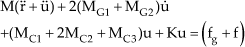
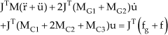
Dynamic equations, after the substitution of the second order differential kinematics equations of the ERLS, can be grouped and rearranged in matrix form, eq.6.

A Rayleigh model of damping has been considered and inserted in the model, i.e., α and β, to deal with realistic flexible industrial robotic systems.

By solving the system Eq. (6), accelerations can be computed and, by means of an appropriate integration scheme, velocities and displacements can be obtained (see [25-26] for more details).

$\begin{array}{l}\left[\begin{array}{l}M MJ\\ J^{T}M J^{T}MJ\end{array}\right]\left[\begin{array}{l}\stackrel{‥}{u}\\ \stackrel{‥}{q}\end{array}\right]=\\ \left[\begin{array}{l}-2\left(M_{G1}+M_{G2}\right)-\alpha M-\beta K -M\stackrel{.}{J} -\left(M_{C1}+2M_{C2}+M_{C3}\right)-K\\ J^T\left(-2\left(M_{G1}+M_{G2}\right)-\alpha M\right) -J^{T}MJ -J^T\left(M_{C1}+2M_{C2}+M_{C3}\right)\end{array}\right]\left[\begin{array}{l}\stackrel{.}{u}\\ \stackrel{.}{q}\\ q\end{array}\right]\\ +\left[\begin{array}{l}M I\\ J^{T}M J^T\end{array}\right]\left[\begin{array}{l}g\\ f\end{array}\right] \end{array}$

(6)

3. Model Validation

3.1. ERLS-FEM simulator

To test this method, a generic Matlab software simulator has been developed accordingly: it exploits the D-H notation and the main concepts of robotics kinematics, allowing us to study the dynamics flexible-link robotic systems without differences with respect to the rigid ones (see Figure.1 where an anthropomorphic robot is considered for simulation, [27,28]).

Figure 1.

Matlab simulator: a) Graphical User Interface (GUI): example of a lightweight anthropomorphic robot simulation.

This simulator is structured in three main parts:

1. D-H, geometrical and mechanical parameters definition.

   Here, the main parameters are inserted in order to unambiguously define the mechanism.

2. Symbolic matrix calculus of the dynamic model and visualization of the mechanism.

   In this phase parameters are checked, first and second order kinematics are computed, and an iterative symbolic algorithm is run to build and save the main matrices of the dynamic formulation. The mechanism's initial configuration is then shown.

3. Dynamic simulation and results evaluation. This means that given the D-H and the mechanical and geometrical parameters of the robotic structure, the simulator is able to compute in an automatic and symbolic way all the terms of the dynamic model. The Simulink Matlab toolbox is then exploited to compute, visualize and save the dynamic behaviour of the robot; simulation time and solver can be directly chosen while external input forces or torques have to be defined in the Simulink environment.

It has to be underlined how the possibility of exploiting such an approach can be very helpful for robot designers both for evaluating the dynamic effects of a structure's change and for accurately computing the elastic displacements of the links.

3.2. Experimental set-up

In this section the experimental set-up that has been realized at the mechatronics laboratory of the Department of Electrical, Management and Mechanical Engineering of the University of Udine is described.

The overall idea was to set-up an experimental system to experimentally validate the ERLS-FEM model and then, in future work, set-up effective model-based controllers for new prototypes of high-performance industrial lightweight robots.

The system hardware, shown schematically in Figure 2, has been set-up in order to have a versatile layout and an easily modifiable structure, thus ready to be integrated with other components for complex prototypes.

Figure 2.

Experimental set-up: a) scheme and b) components

It is composed as follows:

• PC Desktop (PC Target) equipped with:

• Laptop (PC Host).

• Signal Amplifier HBM - KWS3082A and Wheatstone bridge for strain-gauges signal conditioning.

• Drive system Indramat DKC11.1-040-7 FW.

• SPM motor MKD090B-047, 12 Nm.

• Accelerometer PCB 352C65 and signal amplifier PCB 480E09.

The control software was created using the National Instruments Labview 2010 software. In particular, the Real-Time module has been set-up on the Target PC to have a Real Time Operative System (RTOS). The Host PC, connected to the Target PC by means of an Ethernet connection, is devoted to use as a user interface (Figure 3), remote control and data storage and processing. Indeed, through this user interface motion is activated and stopped, and the acquired signals can be analyzed and post-processed. The Real Time control sampling frequency has been set to 1kHz. The implemented control is an open-loop torque control and the torque signal is given to the motor by means of the drive system. The velocity signal comes from the resolver integrated in the back of the motor. Its signal is acquired by the driver system and, as its output, a simulated encoder signal is given.

Figure 3.

L-shape mechanism under test

After the configuration and calibration of the control and acquisition system, an L-shape benchmark mechanism has been set-up to validate the model.

The purpose of this work is to give a first experimental validation of a dynamic modelling approach for 3D robotic systems.

To this end, the particular shape of the system has been chosen: indeed the L-shape configuration allows us to work with a 3D motion of the mechanism, i.e., induce motion and vibrations in different directions and test fast motions under large displacements and small deformations.

In Figure 4 the L-shape mechanism is shown: it is connected to the motor by means of a shrink disk.

Figure 4.

Torque input signal

It is comprised of two flexible rods of aluminium with a square section connected by a rigid aluminium joint and it can be considered as the 3D version of the classic single-link planar mechanism adopted as a benchmark in other approaches limited to 2D motion [19].

The accelerometer is put on the mechanism elbow and strain gauges are installed at the middle points of the links in a half-bridge configuration. Accelerometer and strain-gauge signals are firstly conditioned and amplified by proper devices and then acquired by means of the AD board previously described.

3.3. Results

The input torque signal given to the motor, Figure 4, has been chosen to quickly accelerate and decelerate the mechanism starting from a statically balanced configuration. The L-shape mechanism is driven by two steps in opposite directions. The starting position is 135°, the first step moves the mechanism for about 105°, then the second step is given and the remaining signal stops the motion at about 30°.

The configuration being tested for the L-shape Mechanism is as follows:

• -

  1^st beam: aluminium, L1=0.5m, cross section: 8×8mm

• -

  2^ndbeam: aluminium, L2=0.5 m, cross section:8×8mm

The aluminium's properties are:

• -

  Density: 2700 kg/m³

• -

  Young's modulus 7e10 N/m²

• -

  Poisson's coefficient: 0.33

The simulation has been carried out by using the previously described simulator by considering only two beam elements per part of the L-shape mechanism. The simulated input torque is given in Figure 5 and shows the comparison between the simulated and measured acceleration in the Y coordinate of the last node of the first part of the mechanism, i.e., the elbow, while Figure 6 compares the two signals in the frequency domain.

Figure 5.

Comparison between simulated and measured Y-coordinate accelerations of the elbow node in the time domain

Figure 6.

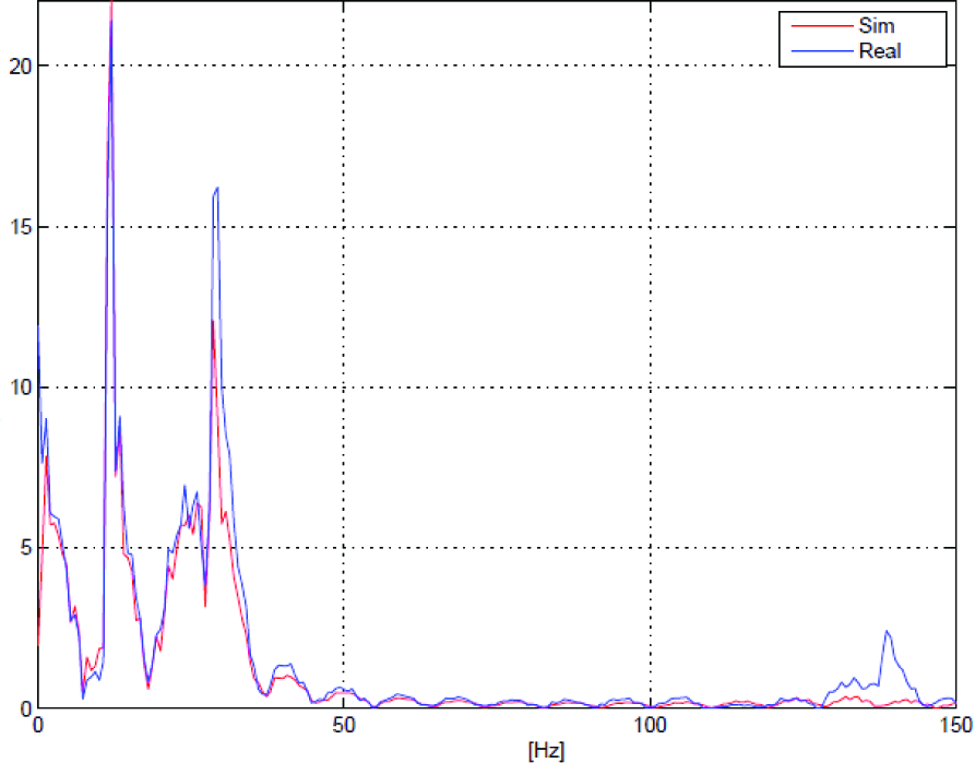
Comparison between simulated and measured Y-coordinate accelerations of the elbow node in the frequency domain

Figure 7 and 8 show the acceleration signal of the last node of the second half of the L-shape mechanism in the time and frequency domain respectively.

Figure 7.

Comparison between simulated and measured Y-coordinate accelerations of the last node of the L-shape mechanism in the time domain

Figure 8.

Comparison between simulated and measured Y-coordinate accelerations of the last node of the L-shape mechanism in the time domain

In Figure 9 the bending moment in the Z local coordinate of the second link obtained by processing the signal acquired from the strain gauges mounted on the central node of the link is shown with respect to time.

Figure 9.

Comparison between simulated and measured bending moment in the Z local coordinate of the second half of the L-shape mechanism in the time domain

Figure 13.

Labview program user interface

As can be seen, the simulated signals match very well with the experimental ones and the main frequencies of the mechanisms are correctly modelled and captured. Indeed, signal amplitudes and vibrational behaviour are captured even if only two beam elements per link have been considered in the simulation.

These results give a first and significant demonstration that the ERLS-FEM approach is effective for modelling a 3D robotic system. Indeed both the gross motion and the elastic behaviour of the mechanical system being tested have been captured. Finally, the approach considered here demonstrates important features that can be useful for industrial robot designers and control engineers since it allows for the maintaining of a classical kinematics approach and, at the same time, the simulation and evaluation of flexible-links robotics systems and their control.

4. Conclusions

In this work, which falls under the general topic of the control of high-dynamics industrial robots both in terms of motion and vibrations, the ERLS-FEM dynamic formulation for flexible-link robots has been considered for experimental validation. This approach can be very useful for industrial robotics and control engineers since it allows us to work with a classical DH formulation, to approach the flexible-link robot as if it were a rigid-link one and, at the same time, take into account the flexibility effects and the coupling between the gross and elastic motion of the overall robotic system.

An experimental set-up has been realized and a 3D L-shape flexible-link mechanism has been tested. The results in terms of acceleration and bending moment signals, i.e., the comparison between the numerical results of a simulator that implements the model under test conditions and the experimental data, are compared showing a good agreement and giving a first and important validation of the approach.

Future work will cover the experimental validation of the model for multi-link robots.