Fuzzy vs Nonfuzzy in 2D Visual Servoing for Robot Manipulators

Abstract

In this paper we consider the tracking control problem of planar robots manipulators via visual servoing in the presence of parametric uncertainties associated with the robot dynamics and the camera parameters. An image–based visual servo control is developed using a Takagi–Sugeno (T–S) fuzzy model. The design includes an image coordinate velocity observer. To the best knowledge of the authors such a proposal remains hitherto unpublished. The new scheme is compared experimentally with two different non–fuzzy algorithms showing the good performance and advantages of the complete system.

1. Introduction

Among the model–based fuzzy control approaches, the Takagi–Sugeno (T–S) is one of the most effective strategies. They proposed their model in 1985 Takagi and Sugeno (1985) and it has emerged as one of the most active areas of research. Basically, a complex dynamic model can be composed in a set of local linear subsystems via fuzzy inference. Hence, it is not surprising that practical applications for control started to appear very quickly after the method had been introduced in different works. On the other hand, in the design of fuzzy controllers a good option is to use parallel distributed compensation (PDC), which offers a procedure to compute a control law from the T–S model. In Kim et al. (2001) a solution to target identification and grasping using a real platform in combination with a vision system is proposed. The task for the robot end–effector is to approach a randomly placed spherical object of known size. The control algorithm is approximated by using an approach based on fuzzy rules that are built in a supervised way, after studying the system behavior. In Wai and Yang (2008) a visual servoing control scheme is proposed for positioning a robot manipulator, divided into two steps: first a fuzzy logic–based visual servoing controller is used to guide the gripper into the neighborhood of the object, and then a local neural network is applied to set the gripper in a desired position. In Fares et al. (2007) a fuzzy logic system and a genetic algorithm are integrated for adaptive visual servoing. Genetic algorithms are employed to optimize the internal parameters of membership functions. In Goncalves et al. (2008) a new uncalibrated eye–to–hand visual servoing based on inverse fuzzy modeling to obtain an inverse relationship of the mapping between image feature variations and joint velocities is proposed. This approach is independent of the robot's kinematic model and camera calibration and avoids the necessity of inverting the manipulator Jacobian online. Different methods can be employed to estimate and identify the internal states of a system when only information from input and output are available, e. g. observer design Tanaka et al. (1998). Fuzzy logic began to be used for the design of observers not long ago, and it is a strategy that is currently under research Zhang and Fei (2006). In Meza (2003) one of the few works on this subject is presented and different designs applied to several nonlinear fuzzy observers are shown with excellent results. In this paper, a fuzzy visual servoing approach for trajectory tracking of planar robot manipulators in the absence of camera parameters, robot dynamics and velocity measurements is introduced. However, on the contrary to the work in Abdelmalek et al. (2007), where a Takagi–Sugeno model based on joint coordinates is employed, in this work we present the model in image coordinates. This strategy is not yet published according to the literature review. Furthermore, an experimental comparison with other well–known algorithms is carried out.

The paper is organized as follows: Section 2 presents the mathematical preliminaries. Section 3 gives the basic concepts about parallel distributed compensation for the Takagi–Sugeno Fuzzy Model and observer design. The control–bserver approach is given in Section 4, while the experimental results are presented in Section 5. Finally, some conclusions are given in Section 6.

2. Preliminaries

The dynamics of a rigid robot arm with revolute joints can adequately be described by using the Euler–Lagrange equations of motion Sciavicco and Siciliano (2000), resulting in

$H\left(q\right)\ddot{q}+C(q,\dot{q})+D\dot{q}+g(q)=\tau -{\tau }_{p^{\prime }}$

(1)

where q ∊ ℝⁿ is the vector of generalized joint coordinates, H(q) ∊ ℝ^n×n is the symmetric positive definite inertia matrix, C(q,q̇)q̇∊ℝⁿ is the vector of Coriolis and centrifugal torques, g(q) ∊ ℝⁿ is the vector of gravitational torques, D ∊ ℝ^n×n is the positive semi definite diagonal matrix accounting for joint viscous friction coefficients, τ ∊ E ℝⁿ is the vector of torques acting at the joints, and τ_p ∊ ℝⁿ represents any bounded external perturbation or friction force.

Throughout this paper, we will assume that the robot is a 2DOF planar manipulator, i. e. it is n = 2 in (1). The direct kinematics is a differentiable map f_k(q):ℝ²→ℝ² relating the joint positions q ∊ ℝ² to the Cartesian position x_R ∊ ℝ² of the centroid of a target attached at the arm end–effector as x_R ∊ f_k (q). In this work we used the camera fixed configuration.

The output of the system is the position y ∊ ℝ² of the image feature, i. e. the position of the target in the computer screen. As shown in Figure 1 the robot workspace is in the x–y plane. The camera is not assumed to be completely parallel to this plane, so that there are two angles of rotation φ,Ψ ∊ ℝ associated to the map from image to workspace coordinates. In order to write y in terms of x_R, the image feature y can be computed through transformation and a perspective projections. As shown in the figure, the following coordinates systems are defined: ∊_o ∊_c·, ∊_c·, ∊_c, ∊_c ∊_c ∊ _i and ∊_y. The position of the origin of the camera frame ∊_C with respect to the robot frame is given by o_C = [o_c1o_c2o_c3]^T. Then, similar to the procedure explained in Kelly and Reyes (2000), by assuming cosψ ≈ 1, sinψ ≈ Ψ, tan Ψ ≈ Ψ, Ψ² ≈ 0 one gets after some manipulation

Figure 1.

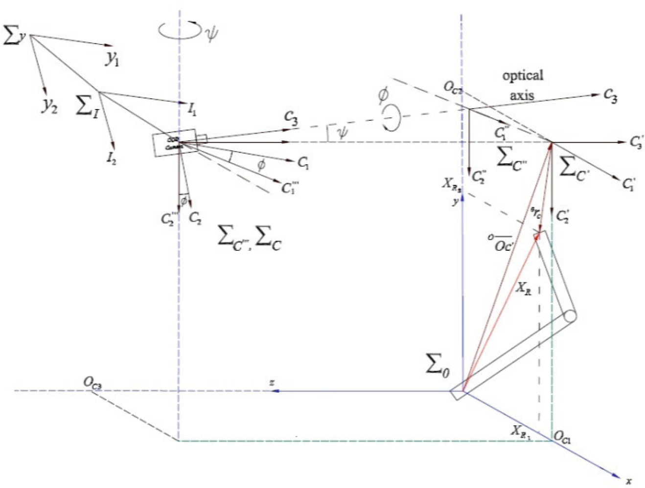
Planar robot system with not parallel camera.

$y={\alpha }_{\lambda }R\phi \left\{x_R-\left[\begin{array}{c}{0}_{c1}\\ 0_{c2}\end{array}\right]\right\}+\left[\begin{array}{c}{u}_0+{\alpha }_{\lambda }\cos (\phi )0_{c3}\psi \\ v_0+{\alpha }_{\lambda }\sin (\phi )0_{c3}\psi \end{array}\right],$

where λ is the focal length, α is a conversion factor from meters to pixels, [u_ov_o]^T is the center offset and

$R_{\phi }=\left[\begin{array}{cc}\cos (\phi )& \sin (\phi )\\ \sin (\phi )& -\cos (\phi )\end{array}\right]$

(2)

3. Parallel distributed compensation for Takagi–Sugeno Fuzzy Model

The parallel distributed compensation (PDC) approach provides a procedure to design a fuzzy controller from a given T–S fuzzy model. The construction of the continuous T–S fuzzy model is based on rules of the form Takagi and Sugeno (1985)

$\begin{array}{l}Rule\text{\hspace{0.17em}i:}If\hspace{0.17em}{z}_1{\text{\hspace{0.17em}is\hspace{0.17em}M}}_{\text{i1}}\text{\hspace{0.17em}and\hspace{0.17em}}\mathrm{...}{\text{and\hspace{0.17em}z}}_{\mathrm{g}}{\text{\hspace{0.17em}is\hspace{0.17em}M}}_{\text{ig}}\\ \text{Then\hspace{0.17em}x}={\mathrm{A}}_{\mathrm{i}}\mathrm{x}\hspace{0.17em}+{\text{\hspace{0.17em}B}}_{\mathrm{i}}\mathrm{u}\\ \mathrm{y}={\mathrm{C}}_{\mathrm{i}}\text{x,\hspace{0.17em}i}=,\text{1,2,\hspace{0.17em}}\mathrm{...}\text{\hspace{0.17em},r}.\end{array}$

(3)

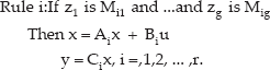
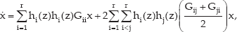
Here M_ij(j = 1,2,…,g) are fuzzy sets, r is the number of model rules, x(t) ∊ ℝⁿ is the system state vector, u(t) ∊ ℝ^m is the input, y(t) ∊ ℝ^q is the output vector, A_i ∊ ℝ^n×n, B_i ∊ ℝ^n×m,C_i ∊ ℝ^q×n,z(t) = [z₁(t),…,z_g(t)] are known premise variables that may be functions of the state variables, external disturbances, and/or time. Given a pair of (x(t),u(t)), a standard fuzzy inference method is used, i. e. a singleton fuzzifier, product fuzzy inference and weighted average defuzzifier. The final state of the fuzzy system is inferred as

$\dot{x}=\frac{{\displaystyle \sum _{i=1}^r{w}_i(z(t))(A_{i}x(t))}}{{\displaystyle \sum _{i=1}^r{w}_i(z(t))}}={\displaystyle \sum _{i=1}^r{h}_i(z(t))(A_{i}x(t)+B_{i}u(t))}$

(4)

$y=\frac{{\displaystyle \sum _{i=1}^r{w}_i(z)C_{i}x}}{{\displaystyle \sum _{i=1}^{r}w{}_i(z)}}={\displaystyle \sum _{i=1}^r{h}_i(z)C_{i}x}$

(5)

where

$w_i((t))={\displaystyle \prod _{j=1}^g{M}_{ij}(z_j(t))}$

(6)

$h_i(z(t))=\frac{w_i(z(t))}{{\displaystyle \sum _{i=1}^r{w}_i(z(t))}}$

(7)

M_ij(z(t)) is the grade of membership of z_j(t) in M_ij. It is assumed that

$w_i(z(t))\ge 0,i=1,2,\mathrm{...},r$

(8)

and

${\displaystyle \sum _{i=1}^r{w}_i(z(t))}>0,$

(9)

for all t. Therefore

$h_i(z(t))\ge 0,i=1,2,\mathrm{...},r$

(10)

and

${\displaystyle \sum _{i=1}^r{h}_i(z(t))=1.}$

(11)

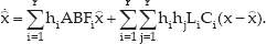
For the convenience of notation h_i(z(t)) = h_i and w_i (z(t)) = w_i. Then the dynamics of the final state of the fuzzy system can be represented as

$\dot{x}(t)={\displaystyle \sum _{i=1}^r{h}_i{A}_{i}x(t)+{\displaystyle \sum _{i=1}^r{h}_i{B}_{i}u}(t).}$

(12)

The main goal is to determine the local feedback gain F_i in the consequent parts. With PDC we have a simple and natural procedure to handle nonlinear control systems. Other nonlinear control techniques require special and rather involved knowledge. The overall output is given by

$u=-{\displaystyle \sum _{i=1}^r{h}_i{F}_{i}x.}$

(13)

The PDC scheme that stabilizes the T–S fuzzy model was proposed by Wang et al. Liu and Lam (2006) as a design framework comprising a control algorithm and a stability test using optimization involving LMI constraints.

3.1 Quadratic Stability Conditions

Consider the following definition.

Definition 3.1. Abdelmalek et al. (2007) The system x(t) = f(x(t),u(t)) is said quadratically stable if there exists a quadratic function V(x(t)) = x^T(t)Px(t),V(0) = 0, called Lyapunov function, satisfying the following conditions

$V(x(t))>0,\hspace{0.17em}\forall x(t)\ne 0\iff P>0,$

(14)

$V(x(t))<0,\hspace{0.17em}\forall x(t)\ne 0$

(15)

By substituting (13) in (4), we obtain the Takagi–Sugeno closed loop fuzzy systems as follows Abdelmalek et al. (2007)

$\dot{x}={\displaystyle \sum _{i=1}^r{\displaystyle \sum _{j=1}^r{h}_i(z)h_j(z)(A_i-B_i{F}_j)x,}}$

(16)

which can be rewritten as

$\dot{x}={\displaystyle \sum _{i=1}^r{h}_i(z)h_i(z)G_{ii}x+2{\displaystyle \sum _{i=1}^r{\displaystyle \sum _{i<j}^r{h}_i(z)h_j(z)\left(\frac{G_{ij}+G_{ji}}{2}\right)x,}}}$

(17)

where G_ij = A_i – B_iF_j and G_ii = A_i – B_iF_i. The stabilization of a feedback system containing a state feedback fuzzy controller has been extensively considered. The stability conditions corresponding to a quadratic Lyapunov function were derived by Tanaka and Sugeno in Tanaka and Sugeno (1992). The approach requires to find a common positive definite matrix for the r subsystems, which makes it very conservative.

3.2 Stabilization Approach

The stabilization approach used in this paper was introduced by Tanaka et al. in Tanaka et al. (2003), where a fuzzy Lyapunov function is proposed. A candidate Lyapunov function is of the form

$V(x(t))={\displaystyle \sum _{i=1}^r{h}_i}(z(t))x^T(t)P_{i}x(t),$

(18)

where P_i is a positive definite matrix and h_i (z(t))≥0, ∊^r_i=1h_i(z(t)) = 1. An interesting advantage is that this form of Lyapunov function takes into account the speed variation of the decision variables, what allows more relaxed stability conditions since this type of functions reduces the global stability of the nonlinear system to the analysis of the local stability of each local linear model (sub–model) separately. The candidate Lyapunov function (18) satisfies the following conditions:

Equation (18) is said to be a fuzzy Lyapunov function for the T–S fuzzy system if the time derivative of V(x(t)) is always negative at x(t) ≠ 0, where P_i is a positive definite matrix. Based on the fuzzy Lyapunov function, we use an approach that gives less conservative stability conditions Abdelmalek et al. (2007), the key assumptions are:

Assumption 3.1. The time derivative of the premise membership function is upper bounded and such that h_i (z(t))≤ φ_i, where φ_i are given positive constants with i = 1, …, r.

Assumption 3.2. The local quadratic Lyapunov functions x^T(t)P_ix(t), i = 1, …, r are proportionally related such that P_j=α_ijP_i for i,j = 1, …,r, where α_ij ≠ 1 and α_ij > 0 for i ≠ j, and α_ij =1 for i = j.

Now consider now the following theorem.

Theorem 3.1. Under Assumptions 3.1 and 3.2, the fuzzy system (16) is stable by using the PDC fuzzy controller (13) if there exist φ_o, α_ij for i,j,ρ = 1, … r, positive definite matrices P₁,P₂, …, P_r and matrices F₁,F₂, …, F_r such that for all i,j,k ∊ {1, …,r}

$P_i>0$

(19)

${\displaystyle \sum _{\rho =1}^r{\phi }_{\rho }{P}_{\rho }+(G_{jj}^T{P}_i+P_i{G}_{jj})<0}$

(20)

${\left(\frac{G_{jk}+G_{kj}}{2}\right)}^T{P}_i+P_i\left(\frac{G_{jk}+G_{kj}}{2}\right)<0(forj<k),$

(21)

where G_jk = A_j – B_jF_k and G_jj = A_j – B_jF_j.

Proof:

The derivative of V(x(t)) in (18) along (17) can be computed after a rather direct but long manipulation as

$\dot{V}(x)=x^T[{\displaystyle \sum _{i=1}^r{\displaystyle \sum _{j=1}^r{h}_i(z)h_j(z)(G_{jj}^T{P}_i+P_i{G}_{jj})+{\displaystyle \sum _{\rho =1}^r{\dot{h}}_{\rho }(z)P_{\rho }}}}+{\displaystyle \sum _{i=1}^r{\displaystyle \sum _{j=1}^r{\displaystyle \sum _{j<k}{h}_i(z)h_j(z)h_k(z)\left({\left(\frac{G_{jk}+G_{kj}}{2}\right)}^T{P}_i+P_i\left(\frac{G_{jk}+G_{kj}}{2}\right)\right)}}}]x$

(22)

$\dot{V}(x)\le x^T[{\displaystyle \sum _{i=1}^r{\displaystyle \sum _{j=1}^r{h}_i{h}_j(G_{jj}^T{P}_i+P_i{G}_{jj})}}+{\displaystyle \sum _{\rho -1}^r{\phi }_{\rho }{P}_{\rho }+}{\displaystyle \sum _{i=1}^r{\displaystyle \sum _{j=1}^r{\displaystyle \sum _{j<k}^{}{h}_i}{h}_j{h}_k\left({\left(\frac{Gjk+Gkj}{2}\right)}^{T}Pi+Pi\left(\frac{Gjk+Gkj}{2}\right)\right)}}]x$

(23)

If Equations (19), (20) and (21) hold, the time derivative of the fuzzy Lyapunov function is negative, i. e. · V(x) ≤ 0, and the closed loop fuzzy system (16) is stable.

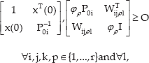
Theorem 3.1 is proven by taking into account Assumption 3.1. The constraint imposed on the time derivative of the premise membership functions and hence on the derivative of the premise variables, i. e. the speed of the state variables for the case of z(t) = x(t), is transformed into LMIs of Theorem 3.2 that are solved simultaneously with those of Theorem 3.1 to stabilize the T–S fuzzy systems. The new LMIs that support Assumption 3.1 allow to increase the performance by limiting the displacement rate in the polytope, implying a facility to find the Lyapunov functions and thus a faster stabilization.

Theorem 3.2. Assumption 3.1 holds if there exist positive definite matrices P₁,P₂, …, P_r and matrices F₁,F₂, …, F_r satisfying

$\begin{array}{l}\left[\begin{array}{cc}1& x^T(0)\\ x(0)& P_i^{-1}\end{array}\right],\left[\begin{array}{cc}{\phi }_{\rho }{P}_i& W_{ij\rho l}^T\\ W_{ij\rho l}& {\phi }_{\rho }I\end{array}\right]\ge O,\end{array}$

(24)

∀i,j,ρ ∊ 1,2, …,r and ∀l, where W_ijρl = ξ_ρl = (A_i – B_iF_j).

Proof:

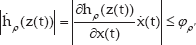
For|̇h_p(z)|≤ø_pand (z = x) one has

$\left|{\dot{h}}_{\rho }(z(t))\right|=\left|\frac{\partial h_{\rho }(z(t))}{\partial x(t)}\dot{x}(t)\right|\le {\phi }_{{\rho }^{\prime }}$

(25)

where

$\frac{\partial h_{\rho }(z(t))}{\partial x(t)}={\displaystyle \sum _{l=1}^s{v}_{\rho l}(z(t)){\xi }_{\rho l},}$

(26)

with ν_ρl ≥ 0 and ∊^s_l=1 ν ρ_l(z(t)) = 1. In (26) ν_ρl (z(t)) depends on the number of membership functions. This term represents the maximum value that each input can have when evaluated in the different functions. ξ_ρl depends on the maximum and minimum values that can take a membership function evaluated at the extreme values of the universe of discourse. This term represents the interval that covers each function. Using (26) we obtain LMIs that satisfy (25), from which we can derive

${\left(\frac{\partial h_{\rho }(z(t))}{\partial x(t)}\dot{x}(t)\right)}^T\left(\frac{\partial h_{\rho }(z(t))}{\partial x(t)}\dot{x}(t)\right)\le {\phi }_{\rho }^2.$

(27)

By replacing (16) in (27) it is

$\frac{1}{{\phi }_{\rho }^2}{x}^T\left[\begin{array}{l}{\left({\displaystyle \sum _{l=1}^s{\upsilon }_{\rho l}{\xi }_{\rho l}\left({\displaystyle \sum _{i=1}^r{\displaystyle \sum _{j=1}^r{h}_i{h}_j[A_i-B_i{F}_j]}}\right)}\right)}^T\\ \left({\displaystyle \sum _{l=1}^s{\upsilon }_{\rho l}{\xi }_{\rho l}\left({\displaystyle \sum _{i=1}^r{\displaystyle \sum _{j=1}^r{h}_i{h}_j[A_i-B_i{F}_j]}}\right)}\right)\end{array}\right]x\le 1.$

(28)

If the fuzzy Lyapunov function (18) satisfies

$V(x(t))\le V(x(0))\le 1,t\ge O,$

(29)

then

$\begin{array}{l}{\displaystyle \sum _{i=1}^r{h}_i(z(t))x^T(t)P_{i}x}(t)\le \\ {\displaystyle \sum _{i=1}^r{h}_i(z(0))x^T}(0)P_{i}x(0)\le 1,\end{array}$

(30)

so that

$1-{\displaystyle \sum _{i=1}^r{h}_i(z(0))x^T(0)P_{i}x(0)\ge O}$

(31)

and

$1-x^T(0)\left({\displaystyle \sum _{i=1}^r{h}_i(z(0))P_i}\right)x(0)\ge O.$

(32)

This last equation can be expressed via LMIs by using the Schur complement as follows:

$\left[\begin{array}{cc}1& x^T(0)\\ x(0)& ({\displaystyle {\sum }_{i=1}^r{h}_i(z(0))P_i{)}^{-1}}\end{array}\right]\ge O,$

(33)

because

$\left[\begin{array}{cc}1& x^T(0)\\ x(0)& P_i^{-1}\end{array}\right]\ge O,fori=1,\mathrm{...},r.$

(34)

This leads to the LMI condition (24). On the other hand, by considering inequalities (28) and (30), inequality (25) holds if

$\begin{array}{l}\frac{1}{{\phi }_{\rho }^2}[\left({\displaystyle \sum _{l=1}^s{\upsilon }_{\rho l}(z){\xi }_{\rho l}\left({\displaystyle \sum _{i=1}^r{\displaystyle \sum _{j=1}^r{h}_i{h}_{j}AB{F}_i^T}}\right)}\right).\\ \left({\displaystyle \sum _{l=1}^s{\upsilon }_{\rho l}(z){\xi }_{\rho l}\left({\displaystyle \sum _{i=1}^r{\displaystyle \sum _{j=1}^r{h}_i{h}_{j}AB{F}_i}}\right)}\right)]\\ -{\displaystyle \sum _{i=1}^r{h}_i{P}_i\le O,}\end{array}$

where $AB{F}_i\stackrel{\mathrm{\Delta }}{=}{A}_i-F_i{F}_j.$ . Equivalently one has

$\left[\begin{array}{cc}{\phi }_{\rho }{\displaystyle {\sum }_{i=1}^r{h}_i{P}_i}& {\displaystyle {\sum }_{l=1}^s{\upsilon }_{\rho l}{\xi }_{\rho l}{Q}^T}\\ {\displaystyle {\sum }_{l=1}^s{\upsilon }_{\rho l}{\xi }_{\rho l}Q}& {\phi }_{\rho }I\end{array}\right]\ge O,$

(35)

where $Q={\displaystyle {\sum }_{i=1}^r{\displaystyle {\sum }_{j=1}^r{h}_i{h}_j\left[A_i-B_i{F}_j\right]}.}$ . This leads to the LMI condition (24).

Remark 3.1. ξ_ρl can be obtained from h_i(z(t)) by using the procedure given in Tanaka and Wang (2001). However, note that the conditions of Theorem 3.2 depend on the initial system state, so that they need to be known.

3.3 Observer Design

In practice, all states may not be fully measurable and it may be necessary to design an observer to implement (13). If the pairs (A_i,C_i) are observable, the fuzzy system (3) is called locally observable. In this work we will assume that this is the case. The design is based on fuzzy implications, with fuzzy sets in antecedents, and a Luenberger observer in the consequents. Each rule is responsible for estimating the states of a locally linear subsystem. The final outputs are obtained by fuzzy blending the local observers outputs. Based on the PDC structure, the local observers are designed as

$\begin{array}{l}Rule\hspace{0.17em}i:if\hspace{0.17em}{z}_1(t)\hspace{0.17em}is\hspace{0.17em}{M}_{i1}\hspace{0.17em}and\hspace{0.17em}\mathrm{...}\hspace{0.17em}and\hspace{0.17em}{z}_g(t)\hspace{0.17em}is\hspace{0.17em}{M}_{ig}\\ Then\hspace{0.17em}\dot{\stackrel{⌢}{x}}=A_i\stackrel{⌢}{x}+B_{i}u+L_i(y-\stackrel{⌢}{y})\\ {\stackrel{⌢}{y}}_i=C_i\stackrel{⌢}{x},\text{\hspace{0.17em}i}=\text{1,2,\hspace{0.17em}}\mathrm{...}\text{\hspace{0.17em},r}\end{array}$

(36)

where L_i with i = 1,2, …, r is the observer gain for the i-th rule. The corresponding PDC fuzzy controller takes form

$u=-{\displaystyle \sum _{i=1}^r{h}_i{F}_i\widehat{x},}$

(37)

instead of (13). Note that the same weight w_i(z) is used. The dependence of the premise variables on the state makes necessary to consider two cases for fuzzy observer design:

1. z₁, …, z_g do not depend on the estimated state

2. z₁,…, z_g depend on the estimated state

In the second case in general h_i(z) ≠ h_i(ẑ) because z ≠ ẑ a priori. Then the premise variables can be the outputs or a combination of the measured states. In this work, we make the following assumption.

Assumption 3.3. z(t) is independent of x.

After Assumption 3.3, it is proposed

$\dot{\stackrel{⌢}{x}}={\displaystyle \sum _{i=1}^r{h}_i[A_i\stackrel{⌢}{x}+B_{i}u+L(y-\stackrel{⌢}{y})]},$

(38)

with final output

$\stackrel{⌢}{y}(t)={\displaystyle \sum _{i=1}^r{h}_i(z(t))C_i\stackrel{⌢}{x}}(t).$

(39)

The design consists in finding the gains L_i in the consequent part, for which it is necessary to compute the observer error dynamics. Substitute (5), (37) and (39) in (38) to obtain

$\dot{\stackrel{⌢}{x}}={\displaystyle \sum _{i=1}^r{h}_{i}AB{F}_i\stackrel{⌢}{x}+{\displaystyle \sum _{i=1}^r{\displaystyle \sum _{j=1}^r{h}_i{h}_j{L}_i{C}_i(x-\stackrel{⌢}{x}).}}}$

(40)

On the other hand, by substituting (37) in system (12) one has

$\dot{x}(t)={\displaystyle \sum _{i=1}^r{\displaystyle \sum _{j=1}^r{h}_i{h}_j(A_{i}x-B_i{F}_j\stackrel{⌢}{x})}}.$

(41)

Define the observer error as

$\stackrel{\sim }{x}=x-\stackrel{⌢}{x}.$

(42)

Then, by subtracting (40) from (41) one gets the observer error dynamics as

$\dot{\stackrel{\sim }{x}}={\displaystyle \sum _{i=1}^r{\displaystyle \sum _{j=1}^r{h}_i{h}_j(A_i-L_i{C}_j)\stackrel{⌢}{x}}.}$

(43)

Now consider the following theorem.

Theorem 3.3. The observer error dynamics (43) is asymptotically stable if there exist positive definite matrices Po₁,P₀₂, …, P_or and matrices L₁,L₂, …, L_r such that the following is satisfied:

$P_{oi}>0$

(44)

$\begin{array}{l}{\displaystyle \sum _{\rho =1}^r{\phi }_{\rho }{P}_{0\rho }+(G_{jj}^T{P}_{0i}+P_{0i}{G}_{jj})}<O\\ {\left(\frac{G_{jk}+G_{kj}}{2}\right)}^T{P}_{0i}+P_{0i}\left(\frac{G_{jk}+G_{kj}}{2}\right)<O\text{for}j<k\end{array}$

(45)

$\begin{array}{c}\left[\begin{array}{cc}1& x^T(0)\\ x(0)& P_{0i}^{-1}\end{array}\right],\left[\begin{array}{cc}{\phi }_{\rho }{P}_{0i}& W_{ij\rho l}^T\\ W_{ij\rho l}& {\phi }_{\rho }I\end{array}\right]\ge O\\ \forall i,j,k,p\in \{1,\mathrm{...},r\}and\forall l,\end{array}$

(46)

where

$G_{jk}=A_j-L_j{C}_{k,}{G}_{jj}=A_j-L_j{C}_{j}and{W}_{ijpl}={\xi }_{pl}(A_i-L_i{C}_j)$

Remark 3.2. By augmenting the states of the system with the state estimation error, we obtain the following 2n dimensional state equations for the observer/controller closed–loop system

$\left[\begin{array}{c}\dot{x}\\ \dot{\stackrel{\sim }{x}}\end{array}\right]=\left[\begin{array}{cc}{\bar{A}}_{11}& {\bar{A}}_{12}\\ 0& {\bar{A}}_{22}\end{array}\right]\left[\begin{array}{c}x\\ \stackrel{\sim }{x}\end{array}\right]$

(47)

$y=\left[\begin{array}{cc}{\displaystyle \sum _{i=1}^r{h}_i{C}_i}& 0\end{array}\right]\left[\begin{array}{c}x\\ \stackrel{\sim }{x}\end{array}\right],$

(48)

With

$A_{11}={\displaystyle {\sum }_{i=1}^r{\displaystyle {\sum }_{j=1}^r{h}_1{h}_1(AB{F}_j),}}\hspace{0.17em}{A}_{12}={\displaystyle {\sum }_{i=1}^r{\displaystyle {\sum }_{j=1}^r{h}_i{h}_j(A_i-L_i{C}_j).}}$

Finally, as shown in Abdelmalek (2009), the separation principle holds for system (4)–(5), so that the error dynamics (47) is asymptotically stable.

4. Visual Servoing Fuzzy Controller Design

Consider a two–link robot arm (see Figure 2). In this section we are interested in a T–S fuzzy model by using PDC laws. The fuzzy controller design is to determine the local feedback gains F_i for the closed loop T–S fuzzy system (16).

Figure 2.

Experimental test bed.

We define X_i = P_i⁻¹, F_i =M_iX_i⁻¹, X_i = α_ijX_j for i,j = 1, …, r, where α_ij ≠ 1 and α_ij > 0 for i ≠ j, and α_ij = 1 for i = j. By giving φ_ρ > 0 and α_ij for i,j,ρ = 1, …, r, we obtain the following LMIs conditions that constitute a stable fuzzy controller design problem:

$X_i>0$

(49)

${\displaystyle \sum _{\rho =1}^r{\phi }_{\rho }{X}_{\rho }+X_i{A}_j^T-{\alpha }_{ij}{M}_j^T{B}_j^T+A_j{X}_i-{\alpha }_{ij}{B}_j{M}_j<O}$

(50)

$\begin{array}{l}{X}_i{A}_j^T-{\alpha }_{ik}{M}_k^T{B}_j^T+X_i{A}_k^T{}_{}-{\alpha }_{ij}{M}_j^T{B}_k^T+\\ +A_j{X}_i-{\alpha }_{ij}{B}_j{M}_k+A_j{X}_i-{\alpha }_{ij}{B}_j{M}_j<O,\end{array}$

(51)

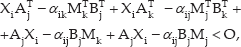
for each set of i,j,k ∊ {1,…,r} such as j < k

$\left[\begin{array}{cc}1& x^T(0)\\ x(0)& X_i\end{array}\right]\ge Ofori=1,\mathrm{...},r,$

(52)

$\left[\begin{array}{cc}{\phi }_{\rho }{X}_i& W_{ij\rho l}^T\\ W_{ij\rho l}& {\phi }_{\rho }I\end{array}\right]\ge O,$

(53)

where W_ijρl = ξ_ρl (A_iX_i – α_ijB_iM_j). Note that from X_i = α_ijX_j we have X_j = (1/α_ij)X_i = α_ijX_i, so that α_ij = 1/ α_ij ∀_i, j ∊ {1, …, r}, and hence, for given i and j, the relation α_ijα_ji = 1 is used. Note that X_i and F_i are computed by solving (13), while M_j can be obtained from these two matrices.

The coefficients α_ij and φ_ρ for i,j,ρ = 1, …, r and i ≠ j, can be chosen heuristically according to the application. In particular, the φ_ρ's are chosen to obtain a fast switching among IF-THEN rules in order to keep the speed of response for a closed–loop system Tanaka and Wang (2001). α_ij and β_ij must be different from 1 (for i = j, α_ij = β_ij = 1) and selection of ξ_ρl is obtained from h_iz(t). Subsequently, we will consider that the premise variables do not depend on the estimated states ○(t). The objective of the tracking control is to make the system outputs follow some predefined trajectories. The inputs are given by the vision system and correspond to the image features, and the output is the torque applied in each joint. The fuzzy observer–based control is summarized as follows

1. Select the fuzzy rules and membership functions for nonlinear system (3).

2. Calculate the matrices A_i, B_i and C_i by using model (3).

3. Establish the reference model or path to follow.

4. Compute L_i.

5. Solve the LMI to obtain F_i.

6. Solve the LMI to obtain P_i.

7. Solve the LMI to obtain P_0i.

8. Construct the fuzzy observer (36).

9. Construct the fuzzy controller (37).

The system state is given by

$\begin{array}{l}x(t)={\left[\begin{array}{cccc}{x}_1& x_2& x_3& x_4\end{array}\right]}^T\\ ={\left[\begin{array}{cccc}{y}_1& y_2& y_3& y_4\end{array}\right]}^T,\end{array}$

(54)

where (Δy₁, Δy₂) represents the robot end–effector position in image coordinates and (Δẏ₁, Δẏ₂) are the corresponding velocities. Note that it is possible to establish the following limits for the state due to physical restrictions.

$\begin{array}{l}{x}_1(t)\in \left[x_{1_{\min }},x_{1_{\max }}\right]=\left[0,1000\right]\left[pixels\right]\\ x_2(t)\in \left[x_{2_{\min }},x_{2_{\max }}\right]=\left[-50,50\right]\left[pixels/s\right]\\ x_3(t)\in \left[x_{3_{\min }},x_{3_{\max }}\right]=\left[0,1000\right]\left[pixels\right]\\ x_4(t)\in \left[x_{4_{\min }},x_{4_{\max }}\right]=\left[-50,50\right]\left[pixels/s\right]\end{array}$

To minimize the design effort and complexity, we try to use as few rules as possible. The maximum and minimum values for state variables are defined based on images acquired. x₁ and x₃ are measurable through the camera. Based on the dynamic model equation which is a function of image coordinates are calculated matrices A_i, B_i and C_i. The T–S fuzzy model is given by the following rules whose membership functions are of triangular form. The premise variables are the tracking error in image coordinates, which is obtained by

$\left[\begin{array}{c}\mathrm{\Delta }{y}_1\\ \mathrm{\Delta }{y}_2\end{array}\right]=\left[\begin{array}{c}{y}_1-y_{d1}\\ y_2-y_{d2}\end{array}\right],$

(55)

where (y₁,y₂) are obtained through the camera image on the computer screen, and (y_d1,y_d2) represent the desired trajectories.

Rule 1: If Δy₁ is about–10 and Δy₂ is about 10 Then Ẋ(t) = A₁x(t) + B₁u(t),y = C₁x(t),

Rule 2: If Δy₁ is about – 10 and Δy₂ is about 0

Then Ẋ(t) = A₂x(t) ₊ B₂u(t),y = C₂x(t),

Rule 3: If Ay₁isabout – 10 and Δy₂ is about – 10 Then Ẋ(t) = A₃x(t) + B₃u(t),y = C₃x(t),

Rule 4: If Δy₁ is about 0 and Δy₂ is about – 10

Then Ẋ(t) = A₄x(t) + B₄u(t),y = C₄x(t),

Rule 5: If Δy₁ is about 0 and Δy₂ is about 0

Then Ẋ(t) = A₅x(t) + B₅u(t),y = C₅x(t),

Rule 6: If Δy₁ is about 0 and Δy₂ is about 10

Then ẋ(t) = A₆x(t)₊B₆u(t),y = C₆x(t),

Rule 7: If Δy₁ is about 10 and Δy₂ is about – 10 Then ẋ (t) = A₇x(t) + B₇u(t),y = C₇x(t),

Rule 8: If Δy₁ is about 10 and Δy₂ is about 0

Then ẋ(t) = A₈x(t)₊B₈u(t),y = C₈x(t),

Rule 9: If Δy₁ is about 10 and Δy₂ is about 10

Then ẋ(t) = A₉x(t)₊B₉u(t),y = C₉x(t).

In order to get the matrices (A_i, B_i,C_i), a model of the form (57) is necessary. In Appendix A a sketch of the robot model in image coordinates, as well as and example of a set (A_i,B_i,C_i), with i = 1, are given. The amount of 9 sets was gotten by trial and error. The image coordinates and their corresponding velocities were considered as the system states, which will be stabilized to zero by the T – S fuzzy controller and observer. The experimental results show that tracking errors tend to zero. The tracking errors are considered in the premise of fuzzy rules; the time derivatives are not considered because the trajectories are small and this does not affect the design of the controller. It is noted that the T-S fuzzy model for the controller and observer design is only an approximation of the robot dynamics given in (57). Therefore, asymptotical stabilization of the fuzzy model does not mean that the original robot dynamics can be asymptotically stabilized, unless the T-S fuzzy model is an exact representation of the original robot dynamics. The number of fuzzy rules allow having a robust system that operates correctly in the operation zone defined. Finally, by employing the MATLAB LMI Toolbox, the corresponding gains F_i and L_i are computed. The results are also shown in the appendix. Note that the MATLAB LMI Toolbox easily allows to satisfy the conditions given in Theorems 3.1, 3.2 and 3.3 to guarantee asymptotical stability of tracking and observation errors.

5. Experimental Results

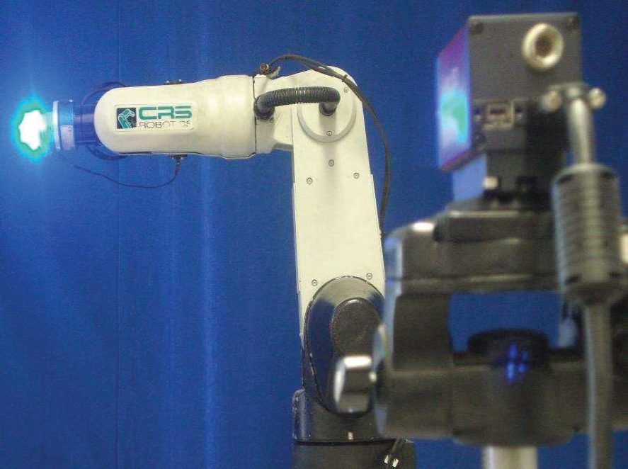
In order to test the theory given in Section 4, the robot A465 of CRS Robotics shown in Figure 2 has been used. It has six degrees of freedom, but only joints 2 and 3 (renumbered 1 and 2, respectively) are employed. The visual system consists of a CCD monochrome camera (Pike F–505B). A circular object is attached to the robot end–effector to recognize it. In order to have a point of comparison, two algorithms have also been programmed. Although they are not explicitly designed to cope with two angles of rotation, we consider that the comparison is fair because both of them are robust schemes.

The Comparative Algorithm 1 is an adaptive second order sliding mode global tracking visual feedback controller developed in Parra-Vega et al. (2003). It has been chosen because it is also meant for planar manipulators in a modified image–based approach. Furthermore, the basic assumption is that the robot model parameters are unknown. The Comparative Algorithm 2 is the one given in Zergeroglu et al. (2001). It is an adaptive calibration controller that compensates for uncertain camera parameters and ensures global asymptotic position tracking. The interested reader can see the reference to check out these schemes, omitted here for lack of room.

5.1 Experimental Outcomes

One experiment has been carried out for all control schemes which is considered representative enough to check out tracking performance. It consists in following a circle in the y₁ – ?y₂ plane described by

$y_d(t)=\left[\begin{array}{c}60\times \sin (0.2t)+650\\ -60\times \cos (0.2t)+450\end{array}\right]\left[pixel\right].$

(56)

With raw eye it was set ø ≈ 45° and Ψ ≈ 25°. Note that the comparative algorithms are only designed for the nominal case Ψ ≈ 0°, thus they rely on their robustness properties to get good results.

In Figure 3, the desired and actual trajectories in the image plane are shown for all approaches. The initial position has been chosen the same in each case and inside the circle. As can be appreciated, the performance appears to be similar in all cases. Note that since the origin (0,0) is in the upper left corner, a minus sign has been added to have the y₂ in the right direction even though it is actually a positive value always. To have a better insight, we have computed the Root Mean Square Error (RMSE) as $\sqrt{\frac{1}{n}{\displaystyle {\sum }_{i=1}^n{e}_i{}^2}}$ where i is the current sample number, e_i is the error associated to i and n is the total number of samples. As can be appreciated in Table 1, the performance of the proposed approach is better. Another advantage of fuzzy logic is that, on the contrary to the adaptive approaches, it does not need any regressor matrix and thus its implementation may be more direct.

Table 1.

Root mean square errors [PIXELS].

Error	Proposed Algorithm	C.Algorithm 1	C.Algorithm 2
Δy1	4.3123	5.7234	5.9960
Δy2	10.7642	15.1442	14.1335

Figure 3.

Trajectory in the image plane (y₁,y₂). Desired trajectory (…). Proposed Algorithm (—). Comp. Algorithm 1 (– –). Comp. Algorithm 2 (- – -).

Finally, the observation errors for the proposed algorithm are shown in Figure 4. While the error s˜₂ becomes zero, s˜₁ has a value of 1[pixel] during more than half the experiment to become zero in the end.

Figure 4.

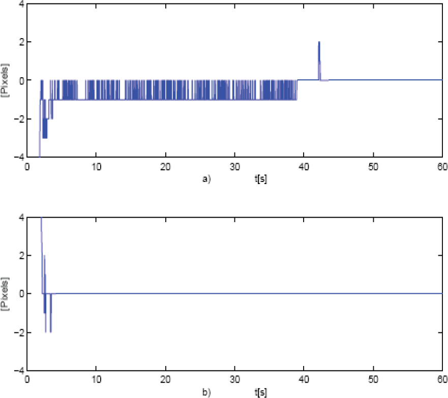
Observer errors for the proposed algorithm. a) s˜₁. b) s˜₂.

6. Conclusions

This paper presents a new fuzzy tracking control scheme for visual servoing applied in a robot manipulator. Based on the T-S model, a fuzzy observer and a fuzzy controller are developed to reduce the tracking errors arbitrarily. Furthermore, the stability of the closed-loop nonlinear system is discussed. The advantage of the proposed tracking control design is that only a simple fuzzy controller is used without feedback linearization or an adaptive scheme. A state space model for a robot manipulator with two degrees of freedom in image coordinates has been suggested which can be employed with other controllers. Experimental results are shown by comparing the proposed scheme with well-known adaptive control laws. The outcomes clearly show the good performance of the algorithm introduced in this work.