Adaptive Formation Control and Collision Avoidance Using a Priority Strategy for Nonholonomic Mobile Robots

Abstract

This paper presents four novel collision avoidance processes for nonholonomic mobile robots to generate effective collision-free trajectories when forming and maintaining a formation. A collision priority strategy integrates the static and dynamic collision priorities to avoid a collision efficiently and effectively. In addition, it minimizes the turning angle of the follower robot and decreases system computation time. When avoiding collisions between robots, a novel collision avoidance algorithm is used to find a safe waypoint for the robot, based on the velocity of each robot. An adaptive tracking control algorithm, using the Lyapunov analysis, guarantees that the robot's trajectory and velocity tracking errors converge to zero considering parametric uncertainties of both the kinematic and dynamic models. The simulation and experiment results validate the effectiveness of the proposed method.

1. Introduction

Over the past decades, multi-robot formation forming and maintaining has been regarded as a major topic of interest because of its benefits of feasibility, accuracy, robustness and flexibility. The existing formation control approaches include the behaviour-based approach [1], the virtual structure approach [2, 3] and the leader-follower approach [4, 5]. Due to its easiness to understand and implement, the leader-follower approach has stimulated a great deal of research. When using the leader-follower approach, one or more robots are designated as the leader robots, while the follower robots keep track of the leader robots to form and maintain the formation.

Collision avoidance control is a problem in multi-robot formation systems. To solve this problem, four collision avoidance processes are presented, consisting of collision detection, collision judgement, collision priority and the collision avoidance algorithm. This paper focuses on the third and fourth processes.

With respect to a collision priority process, a static collision priority strategy is coordinated using a dynamic collision priority strategy. Firstly, after avoiding the collisions, a block in reforming formation may happen, that may cause a deadlock problem increasing the collision avoidance trajectory. Therefore, the static collision priority strategy is proposed to increase the efficiency and effectiveness of the collision avoidance. Secondly, when designing the trajectory for the robot, the term ‘smooth’ is an essential point to be considered. If the robot turns 90 degrees in a time step, the guarantee of smooth trajectory is impossible, and the wheels of the robot slip easily, causing the increase of localization errors for the robot. Hence, the follower robot minimizes the turning angle using the proposed dynamic collision priority strategy in this paper. In addition, since the dynamic collision priority is based on the actual situation during the motions, the computation time is increased within the system. The solution to this problem will be outlined in section 3.

The documented priority strategy studies are as follows. Using the global knowledge, [6-8] propose the static priority strategy, where the priority is assigned to each robot beforehand and cannot be changed during the motion. The dynamic priority strategy in [9] is based on occupancy of local searching space, where each robot recalculates its priority and exchanges the information with its nearby robot, but the strategy cannot solve the disorder and deadlock problem. In [10], the dynamic priority is introduced, where the network structure is presented based on the motion conflicts amongst the robots. However, there are difficulties in establishing a conflict graph, which includes all robots in the system, at each time step.

The proposed collision priority strategy has the following attributes. (1) The static collision priority is related to the formation model and it is very simple; (2) the proposed dynamic collision priority aims to obtain a smooth trajectory by minimizing the turning angle of the follower robot; and (3) due to the integration of the static and dynamic collision priorities, the follower robot does not need to calculate the priorities continuously, while avoiding collisions. Hence, the computation and the complexity of the system can be extensively decreased.

With respect to a collision avoidance algorithm process, a novel collision avoidance algorithm is coordinated with multi-robot formation, based on the velocity and velocity orientation of each robot. In other research, the artificial potential method has been widely used to plan a collision-free path, where the motion of the robot is controlled by the negative gradient of a mixture of attractive and repulsive potential functions as control inputs. However, since the path is described in the form of a high order polynomial, the computations referring to the analytical motion planning are complex and even unsolvable [2]. The dynamic motion planning method to deal with the collision avoidance problem is also used in [11, 12], requiring full knowledge of the obstacle's trajectory.

Motion control is another important function in multi-robot systems. The trajectory tracking problem is widely solved using the kinematic model of a mobile robot [13-15], where ‘perfect velocity’ tracking is assumed to generate the actual velocity control inputs. However, since it is difficult for the dynamics of the robot to produce the perfect velocity as the kinematic controller [16], the torque input is used [17]. This paper presents an adaptive tracking control algorithm which integrates an adaptive kinematic controller and a torque controller for the nonholonomic mobile robot, based on [18, 19].

This paper is organized as follows. Section 2 gives three research models. Section 3 discusses the four collision avoidance control processes. Section 4 outlines the robust adaptive controllers. Section 5 shows the simulation results. Finally, in section 6, the experimental results are presented.

2. Research Models

2.1 A Nonholonomic Mobile Robot Model

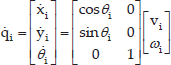
The nonholonomic mobile robot is shown in Fig. 1. The robot R_i (i is the robot number i = 1,2,…,N) consists of a passive wheel and two actuated wheels (e.g., DC motor) to achieve the motion and orientation. The radius of both of the actuated wheels is r_i. The distance between the two actuated wheels is denoted by 2b_i. The centre of mass of the mobile robot is located at P_ic, and P_io is located in the middle point between the right and left driving wheels. The distance between P_ic and P_io is denoted by d_i. {o,x,y} is an inertial Cartesian and {P_ic,X,Y} is the local frame fixed on the robot. Three generalized coordinates of the robot configuration can be described as q_i = [x_i,y_i,0θ_i]^T in an inertial Cartesian frame, where (x_i,y_i) are the coordinates of the point P_ic in the inertial Cartesian frame and θ_i is the orientation of the basis {P_ic,X,Y} with respect to the inertial basis. Define v_i and ω_i as the linear and angular velocities of the robot, the ordinary form of the robot R_i kinematic model is as (1).

Figure 1.

Two-wheeled nonholonomic mobile robot model

${\dot{q}}_{\mathrm{i}}=\left[\begin{array}{c}{\dot{x}}_{\mathrm{i}}\\ {\dot{y}}_{\mathrm{i}}\\ {\dot{\theta }}_{\mathrm{i}}\end{array}\right]=\left[\begin{array}{cc}\cos {\theta }_{\mathrm{i}}& 0\\ \sin {\theta }_{\mathrm{i}}& 0\\ 0& 1\end{array}\right]\left[\begin{array}{c}{\mathrm{v}}_{\mathrm{i}}\\ {\omega }_{\mathrm{i}}\end{array}\right]$

(1)

Define v_i = (y_i1 ,v_i2)^T as the angular velocities of the right and left wheels of the robot R_i. The relationship between v_i, ω_i and v_i1 ,v_i2 is as follows.

${\nu }_{\mathrm{i}}=\left[\begin{array}{c}{\nu }_{\mathrm{i}1}\\ {\nu }_{\mathrm{i}2}\end{array}\right]=\frac{1}{{\mathrm{r}}_{\mathrm{i}}}\left[\begin{array}{cc}1& {\mathrm{b}}_{\mathrm{i}}\\ 1& -{\mathrm{b}}_{\mathrm{i}}\end{array}\right]\left[\begin{array}{c}{\mathrm{v}}_{\mathrm{i}}\\ {\omega }_{\mathrm{i}}\end{array}\right]$

(2)

The robot can only move in the direction normal to the axis of the driving wheels, and the wheels do not slip. Define φ_ir and φ_i1 as the angles of the right and left driving wheels of the robot R_i. These nonholonomic constraints can be written as (3)-(5).

${\dot{y}}_{\mathrm{i}}\cos {\theta }_{\mathrm{i}}-{\dot{x}}_{\mathrm{i}}\sin {\theta }_{\mathrm{i}}=0$

(3)

${\dot{x}}_{\mathrm{i}}\cos {\theta }_{\mathrm{i}}+{\dot{y}}_{\mathrm{i}}\sin {\theta }_{\mathrm{i}}+{\mathrm{b}}_{\mathrm{i}}{\dot{\theta }}_{\mathrm{i}}={\mathrm{r}}_{\mathrm{i}}{\dot{\phi }}_{ir}$

(4)

${\dot{x}}_{\mathrm{i}}\cos {\theta }_{\mathrm{i}}+{\dot{y}}_{\mathrm{i}}\sin {\theta }_{\mathrm{i}}-{\mathrm{b}}_{\mathrm{i}}{\dot{\theta }}_{\mathrm{i}}={\mathrm{r}}_{\mathrm{i}}{\dot{\phi }}_{il}$

(5)

Since the trajectory of the mobile robot base is constrained to the horizontal plane, the gravitational vector G(q) is zero. The motion of the nonholonomic mobile robot R_i are given by

${\dot{q}}_{\mathrm{i}}=\mathrm{S}({\mathrm{q}}_{\mathrm{i}}){\nu }_{\mathrm{i}}(\mathrm{t})$

(6)

$\bar{M}({\mathrm{q}}_{\mathrm{i}}){\dot{\nu }}_{\mathrm{i}}+\bar{V}({\mathrm{q}}_{\mathrm{i}},{\dot{q}}_{\mathrm{i}}){\nu }_{\mathrm{i}}+{\bar{\tau }}_{id}=\bar{B}{\tau }_{\mathrm{i}}$

(7)

In these expressions, τ_i = (τ_i1,τ_i2)^T is the torque applied on the robot R_i 's right and left wheels. m_ic and m_iw are the mass of the body and wheel with a motor. I_ic, I_iw, and I_im are the moment of inertia of the body with respect to the vertical axis through P_ic, the wheel with a motor with respect to the wheel axis, and the wheel with a motor with respect to the wheel diameter, respectively. τ_id is the bounded unknown disturbances of robot R_i including unstructured and unmodelled dynamics.

Property 1:M̄(q_i) is symmetric and positive definite.

Property 2: $(\dot{\stackrel{̄}{M}}-2\bar{V})$ is skew symmetric.

Assumption 1: The bounded disturbances ${\bar{\tau }}_{id}$ satisfies $\Vert {\bar{\tau }}_{id}\Vert \le c_{i0}+c_{i1}\Vert {\nu }_i\Vert$ , with positive constants $c_{i0}$ and $c_{i1}$ [19].

2.2 The Leader-Follower Formation Model

In the formation control method, n robots are controlled to move in a stable mode. A robot is assigned to be the leader robot, which determines the follower robot's motion by defining the desired distance and the desired bearing angle. The follower robot calculates the waypoint by the desired distance and the desired bearing angle.

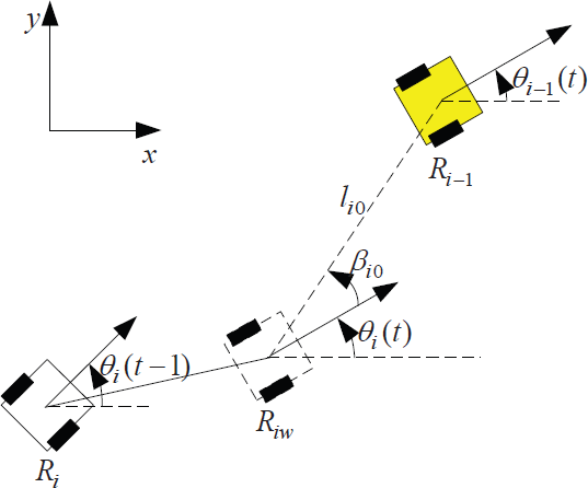
Let R_i-1 and R_i be the leader robot and the follower robot, respectively. l_i is denoted as the actual distance between R_i-1 and R_i, l_i0 as the desired distance. β_i is denoted as the actual bearing angle from the orientation of the follower robot to the axis connecting R_i-1 and R_i, and β_i0 as the desired bearing angle. The formation for the leader robot R_i-1 -waypointR_iw -the follower robot R_i with the desired distance and the desired bearing angle is shown in Fig.2, where θ_i (t) = θ_i-1 (t). The waypoint of the follower robot R_i is denoted by q_iw = (x_iw,y_iw θ_iw)^T as (8).

Figure 2.

The leader-follower formation model

$\left[\begin{array}{c}{\mathrm{x}}_{iw}(\mathrm{t})\\ {\mathrm{y}}_{iw}(\mathrm{t})\\ {\theta }_{iw}(\mathrm{t})\end{array}\right]=\left[\begin{array}{c}{\mathrm{x}}_{\mathrm{i}-1}(\mathrm{t})-{\mathrm{l}}_{\mathrm{i}0}\cos ({\beta }_{\mathrm{i}0}+{\theta }_{\mathrm{i}}(\mathrm{t}))\\ {\mathrm{y}}_{\mathrm{i}-1}(\mathrm{t})-{\mathrm{l}}_{\mathrm{i}0}\sin ({\beta }_{\mathrm{i}0}+{\theta }_{\mathrm{i}}(\mathrm{t}))\\ {\theta }_{\mathrm{i}-1}(\mathrm{t})\end{array}\right]$

(8)

2.3 The Follower Robot Control Model

The collision-free trajectory of the leader robot is predefined and the follower robots track the leader robot while avoiding the collisions. Fig. 3 shows the block diagram to control the follower robot. The follower robot communicates with the leader robot and checks possible collisions with other follower robots. If there is collision danger, the collision judgement process decides whether or not the follower robot starts a collision avoidance algorithm. Based on the waypoint from formation control or collision avoidance control, the adaptive controllers are calculated for the follower robot.

Figure 3.

The block diagram of the follower robot control

3. The Collision Avoidance Control

In this section, follower robots try to complete a collision avoidance task in forming and maintaining formation with a leader robot effectively and efficiently. The task includes four processes: collision detection, collision judgement, collision priority and the collision avoidance algorithm. The four processes are detailed as follows.

3.1 The Collision Detection

Let R_i and R_j denote two follower robots, with their states as (x_i,y_i,θ_i)^T and (x_j,y_j,θ_j)^T, respectively. The distance D_ij between two follower robots is shown in (9).

${\mathrm{D}}_{ij}=\sqrt{{({\mathrm{x}}_{\mathrm{i}}-{\mathrm{x}}_{\mathrm{j}})}^2+{({\mathrm{y}}_{\mathrm{i}}-{\mathrm{y}}_{\mathrm{j}})}^2}$

(9)

As shown in Fig. 4, based on moving speed and physical size of the follower robot, two pseudo protected shells are defined surrounding the follower robot R_i and R_j, with the radius of s_i and s_j, respectively. If the distance D_ij satisfies the Equation (10), the two follower robots must consider the collision avoidance.

Figure 4.

The protected shells of follower robot R_i and R_j

${\mathrm{D}}_{ij}=\sqrt{{({\mathrm{x}}_{\mathrm{i}}-{\mathrm{x}}_{\mathrm{j}})}^2+{({\mathrm{y}}_{\mathrm{i}}-{\mathrm{y}}_{\mathrm{j}})}^2}\le ({\mathrm{s}}_{\mathrm{i}}+{\mathrm{s}}_{\mathrm{j}})$

(10)

3.2 The Collision Judgement

After detecting a collision, the follower robots judge whether to start the collision avoidance algorithm or not, based on the method in [20]. The judgement of a collision danger relies on the distance D_ij (t) and its derivative dD_ij (t) / dt. As the classifications in Table 1, if the collision danger increases, the two follower robots are required access to the collision avoidance algorithm.

Table 1.

The two follower robots collision danger with respect to D_ij (t)anddD_ij (t) / dt.

Case	Dij (t)	dDij (t) / dt	Collision danger
1	Dij (t) ≤ (si + sj)	> 0	Danger decreases.
2	Dij (t) ≤ (si + sj)	≤ 0	Danger increases.

3.3 The Collision Priority

Following the collision detection and the collision judgement processes, to avoid collision efficiently and effectively, and to minimize the turning angle of the follower robot, there are two main considerations: 1. Which follower robot should be selected to apply the collision avoidance algorithm; 2. Which follower robot should continue tracking the formation. Therefore, in the collision priority process, the static priority is integrated with the dynamic priority to select which follower robot will perform the collision avoidance algorithm.

3.3.1 The static priority

After avoiding the collisions, due to the longer desired distance with the leader robot, the follower robot may block other follower robots from reforming the formation. Hence, a collision may occur again, causing the increase of the collision avoidance trajectory and the deadlock problem. To overcome these problems, the static priority p^s_i (i is the robot number i = 1,2,…,N) for each follower robot is initially defined. The value of the static priority is given by the reciprocal of the desired distance l_i0 with the leader robot as (11).

${\mathrm{p}}_{\mathrm{i}}^{\mathrm{s}}=1/{\mathrm{l}}_{\mathrm{i}0}$

(11)

From (11), if the desired distance of the follower robot R_j with the leader robot is shorter than the follower robot R_i, p^s_j is higher than p^s_i. If the desired distances of the two follower robots R_i and R_j are the same, p^s_i = p^s_j.

3.3.2 The dynamic priority

To minimize the turning angle of the follower robot, a dynamic priority strategy is introduced to give orders to the robots. Based on the collision avoidance algorithm, define the dynamic priority p^d_i (i is the robot number, i = 1,2,…,N) function

${\mathrm{p}}_{\mathrm{i}}^{\mathrm{d}}={\displaystyle {\sum }_{\mathrm{j}=1}^{\mathrm{n}(\mathrm{j}\ne \mathrm{i})}{\lambda }_{\mathrm{j}}\mathrm{p}\hspace{0.17em}},\hspace{0.17em}{\lambda }_{\mathrm{j}}=\{\begin{array}{ll}0\hfill & {\theta }_{\mathrm{i}}<{\theta }_{\mathrm{j}}\hfill \\ 1\hfill & {\theta }_{\mathrm{i}}\ge {\theta }_{\mathrm{j}}\hfill \end{array}$

(12)

where θ_i and θ_j are estimated turning angles of the follower robot R_i and R_j, respectively, based on the collision avoidance algorithm. pis a positive constant in (12). If the follower robots share the same static priority, the dynamic priority approach is used to choose the follower robot for addressing the collision avoidance algorithm. If there are multiple robots, the term p^d_i = Σ^n(j≠i)_j=1 λ_j p mean s the accumulation of all turning angle comparisons between the follower robot R_i and the other follower robot R_j (j = 1,2,…,N, j ≠ i).

3.3.3 The cooperation of the static and dynamic priorities

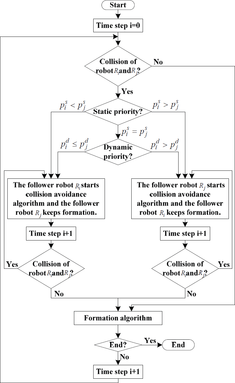
In order to increase collision avoidance efficiency and minimize the robot's turning angle, the follower robot is selected to apply the collision avoidance algorithm, based on the cooperation of the static and dynamic priorities. The cooperation flowchart is illustrated in Fig. 5.

Figure 5.

The cooperation flowchart of the static and the dynamic collision priorities

After the collision detection and judgement processes, the follower robot is chosen to avoid the collision via the following steps. Firstly, the selection of whether to implement the collision avoidance algorithm or to keep the formation is based on the comparison between the static priorities of the follower robots. If p^s_i > p^s_j, the follower robot R_i continues tracking the formation, and the follower robot R_j goes into the collision avoidance algorithm process. Secondly, if the static priorities of the follower robots are the same, the follower robot is chosen to implement the collision avoidance algorithm by the comparison result of the dynamic priorities. If p^d_i > p^d_j, the follower robot R_j starts the collision avoidance algorithm, while the follower robot R_i follows the leader robot. Thirdly, if the follower robots continue to have the collision avoidance problem, the follower robot directly applies the collision avoidance algorithm with the selection from steps 1 and 2. In this way, the calculation and the comparison time can be decreased by skipping the comparison of the static and dynamic collision priorities.

3.4 The Collision Avoidance Algorithm

The collision avoidance algorithm is presented in Fig.6. Referring to the collision detection process, the collision judgement process and the collision priority process, the follower robot R_i is assumed to avoid collision with the follower robot R_j. As shown in Fig.6, the follower robot R_i and R_j are currently located at A and B, with the position state P_i = (x_i,y_i)^T and P_j = (x_j,y_j)^T, respectively. α₁ is the angle from the axis x to the axis AB.

Figure 6.

The collision avoidance algorithm of the follower robot R_i

${\alpha }_1=\arctan \left(\frac{{\mathrm{y}}_{\mathrm{j}}-{\mathrm{y}}_{\mathrm{i}}}{{\mathrm{x}}_{\mathrm{j}}-{\mathrm{x}}_{\mathrm{i}}}\right)$

(13)

Define |θ_j – θ_i | as the relative angle of the orientation of the follower robots R_i and R_j, the angle α₂ is written as (14). For the velocities of R_i and R_j given by Ṗ_i and Ṗ_j, the angle α₃ is denoted as (15).

${\alpha }_2=\pi -|{\theta }_{\mathrm{j}}-{\theta }_{\mathrm{i}}|$

(14)

${\alpha }_3=\arccos \left(\frac{{\dot{P}}_{\mathrm{i}}-{\dot{P}}_{\mathrm{j}}\cos {\alpha }_2}{\sqrt{{({\dot{P}}_{\mathrm{i}})}^2+{({\dot{P}}_{\mathrm{j}})}^2-2{\dot{P}}_{\mathrm{i}}{\dot{P}}_{\mathrm{j}}\cos {\alpha }_2}}\right)$

(15)

α₄ is the angle between the orientation of the follower robot R_i and the axis AB at point A. The angle α₄ can be calculated as (16).

${\alpha }_4=|{\theta }_{\mathrm{i}}-{\alpha }_1|$

(16)

The goal of the collision avoidance algorithm is to enlarge the distance between the follower robots until the distance is equal to the sum of the protected shell radius of the follower robots (s_i + s_j). Considering the smoothness of the trajectory, the waypoint for follower robot R_i is located at C to satisfy the requirement |θ_i (t) – θ(t – 1) |< ∂ / 2. The distance of AC is calculated as

${\mathrm{r}}_{wp}={\mathrm{D}}_{ij}\cos {\alpha }_5+\sqrt{{({\mathrm{s}}_{\mathrm{i}}+{\mathrm{s}}_{\mathrm{j}})}^2-{\mathrm{D}}_{ij}^2{\sin }^2{\alpha }_5}$

(17)

where α₅ = α₃ + α₄. For the parameters discussed above, the waypoint equation to avoid collision is given by

$\left[\begin{array}{c}{\mathrm{x}}_{iw}(\mathrm{t})\\ {\mathrm{y}}_{iw}(\mathrm{t})\\ {\theta }_{iw}(\mathrm{t})\end{array}\right]=\left[\begin{array}{c}{\mathrm{x}}_{\mathrm{i}}(\mathrm{t}-1)+{\mathrm{r}}_{wp}\cos ({\theta }_{\mathrm{i}}(\mathrm{t}-1)\pm {\alpha }_3)\\ {\mathrm{y}}_{\mathrm{i}}(\mathrm{t}-1)+{\mathrm{r}}_{wp}\sin ({\theta }_{\mathrm{i}}(\mathrm{t}-1)\pm {\alpha }_3)\\ {\theta }_{\mathrm{i}}(\mathrm{t}-1)\pm {\alpha }_3\end{array}\right]$

(18)

where r is the distance to move for the next step and θ_i (t – 1) ± α₃ is the angle to turn. Based on the orientation of the follower robot R_i, note that when the follower robot R_j is on the right-side of the follower robot R_i, select θ_i (t – 1) + α₃ in (18), otherwise, select θ_i (t – 1) – α₃.

4. Robust Adaptive Controllers Design

In this section, adaptive controllers are designed for the robot with two actuated wheels based on kinematic and dynamic models. The designed controller can guarantee that the robot's trajectory and velocity tracking errors converge to zero asymptotically stably under the parametric uncertainties of the kinematic and dynamic models.

4.1 Adaptive Control of the Kinematic Model

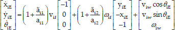
Considering the kinematic model in (6), an adaptive tracking controller for the kinematic part is designed based on [18]. The waypoint equations are defined as

${\dot{x}}_{iw}={\mathrm{v}}_{iw}\cos {\theta }_{iw}$

(19)

${\dot{y}}_{iw}={\mathrm{v}}_{iw}\sin {\theta }_{iw}$

(20)

${\dot{\theta }}_{iw}={\omega }_{iw}$

(21)

where v_iw and ω_iw are the waypoint input. Comparing the waypoint state q_iw with the current measured state q_ic, the tracking error posture can be described as (22).

${\mathrm{E}}_{iq}=\left[\begin{array}{c}{\mathrm{x}}_{iE}\\ {\mathrm{y}}_{iE}\\ {\theta }_{iE}\end{array}\right]=\left[\begin{array}{ccc}\cos {\theta }_{ic}& \sin {\theta }_{ic}& 0\\ -\sin {\theta }_{ic}& \cos {\theta }_{ic}& 0\\ 0& 0& 1\end{array}\right]\left[\begin{array}{c}{\mathrm{x}}_{iw}-{\mathrm{x}}_{ic}\\ {\mathrm{y}}_{iw}-{\mathrm{y}}_{ic}\\ {\theta }_{iw}-{\theta }_{ic}\end{array}\right]$

(22)

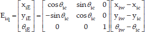
The derivative matrix Ė_iq can be derived as (23).

${\dot{E}}_{iq}=\left[\begin{array}{c}{\dot{x}}_{iE}\\ {\dot{y}}_{iE}\\ {\dot{\theta }}_{iE}\end{array}\right]=\left[\begin{array}{c}-1\\ 0\\ 0\end{array}\right]{\mathrm{v}}_{ic}+\left[\begin{array}{c}{\mathrm{y}}_{iE}\\ -{\mathrm{x}}_{iE}\\ -1\end{array}\right]{\omega }_{ic}+\left[\begin{array}{c}{\mathrm{v}}_{iw}\cos {\theta }_{iE}\\ {\mathrm{v}}_{iw}\sin {\theta }_{iE}\\ {\omega }_{iw}\end{array}\right]$

(23)

Based on [18], the linear and angular velocity v_ic and ω_ic are given as v_if and ω_if, respectively,

$\left[\begin{array}{c}{\mathrm{v}}_{if}\\ {\omega }_{if}\end{array}\right]=\left[\begin{array}{c}{\mathrm{v}}_{iw}\cos {\theta }_{iE}+{\mathrm{K}}_{\mathrm{i}1}{\mathrm{x}}_{iE}\\ {\omega }_{iw}+{\mathrm{K}}_{\mathrm{i}2}{\mathrm{v}}_{iw}{\mathrm{y}}_{iE}+{\mathrm{K}}_{\mathrm{i}3}\sin {\theta }_{iE}\end{array}\right]$

(24)

where K_i1, K_i2, and K_i3 are positive constants. Using (2), (23) is transformed to

$\left[\begin{array}{c}{\dot{x}}_{iE}\\ {\dot{y}}_{iE}\\ {\dot{\theta }}_{iE}\end{array}\right]=\left[\begin{array}{c}-\frac{{\mathrm{r}}_{\mathrm{i}}}{2}+\frac{{\mathrm{r}}_{\mathrm{i}}}{2{\mathrm{b}}_{\mathrm{i}}}{\mathrm{y}}_{iE}\\ -\frac{{\mathrm{r}}_{\mathrm{i}}}{2{\mathrm{b}}_{\mathrm{i}}}{\mathrm{x}}_{iE}\\ -\frac{{\mathrm{r}}_{\mathrm{i}}}{2{\mathrm{b}}_{\mathrm{i}}}\end{array}\right]{\nu }_{\mathrm{i}1}+\left[\begin{array}{c}-\frac{{\mathrm{r}}_{\mathrm{i}}}{2}-\frac{{\mathrm{r}}_{\mathrm{i}}}{2{\mathrm{b}}_{\mathrm{i}}}{\mathrm{y}}_{iE}\\ \frac{{\mathrm{r}}_{\mathrm{i}}}{2{\mathrm{b}}_{\mathrm{i}}}{\mathrm{x}}_{iE}\\ \frac{{\mathrm{r}}_{\mathrm{i}}}{2{\mathrm{b}}_{\mathrm{i}}}\end{array}\right]{\nu }_{\mathrm{i}2}+\left[\begin{array}{c}{\mathrm{v}}_{iw}\cos {\theta }_{iE}\\ {\mathrm{v}}_{iw}\sin {\theta }_{iE}\\ {\omega }_{iw}\end{array}\right]$

(25)

If the parameters r_i and b_i are not known, the angular velocities of the left and right wheels cannot be obtained by the linear and angular velocities in (2). Based on [19], set a_i1 = 1/r_i and a_i2 = b_i /r_i, v_i1 and v_i2 are chosen as

${\nu }_{ic}=\left[\begin{array}{c}{\nu }_{\mathrm{i}1\mathrm{c}}\\ {\nu }_{\mathrm{i}2\mathrm{c}}\end{array}\right]=\left[\begin{array}{cc}{\widehat{a}}_{\mathrm{i}1}& {\widehat{a}}_{\mathrm{i}2}\\ {\widehat{a}}_{\mathrm{i}1}& -{\widehat{a}}_{\mathrm{i}2}\end{array}\right]\left[\begin{array}{c}{\mathrm{v}}_{if}\\ {\omega }_{if}\end{array}\right]=\left[\begin{array}{cc}{\mathrm{a}}_{\mathrm{i}1}+{\stackrel{\sim }{a}}_{\mathrm{i}1}& {\mathrm{a}}_{\mathrm{i}2}+{\stackrel{\sim }{a}}_{\mathrm{i}2}\\ {\mathrm{a}}_{\mathrm{i}1}+{\stackrel{\sim }{a}}_{\mathrm{i}1}& -{\mathrm{a}}_{\mathrm{i}2}-{\stackrel{\sim }{a}}_{\mathrm{i}2}\end{array}\right]\left[\begin{array}{c}{\mathrm{v}}_{if}\\ {\omega }_{if}\end{array}\right]$

(26)

where ǎ_i1 and ǎ_i2 are the estimate of a_i1 and a_i2, and ã_i1 = ǎ_i1 – a_i1, ã_i2 = ǎ_i2 – a_i2. (25) can be described as (27).

$\left[\begin{array}{c}{\dot{x}}_{iE}\\ {\dot{y}}_{iE}\\ {\dot{\theta }}_{iE}\end{array}\right]=\left(1+\frac{{\stackrel{\sim }{a}}_{\mathrm{i}1}}{{\mathrm{a}}_{\mathrm{i}1}}\right){\mathrm{v}}_{if}\left[\begin{array}{c}-1\\ 0\\ 0\end{array}\right]+\left(1+\frac{{\stackrel{\sim }{a}}_{\mathrm{i}2}}{{\mathrm{a}}_{\mathrm{i}2}}\right){\omega }_{if}\left[\begin{array}{c}{\mathrm{y}}_{iE}\\ -{\mathrm{x}}_{iE}\\ -1\end{array}\right]+\left[\begin{array}{c}{\mathrm{v}}_{iw}\cos {\theta }_{iE}\\ {\mathrm{v}}_{iw}\sin {\theta }_{iE}\\ {\omega }_{iw}\end{array}\right]$

(27)

To design ǎ_i1 and ǎ_i2, based on [21], the Lyapunov function is chosen as (28), where ${\dot{\stackrel{\sim }{a}}}_{i1}={\dot{\widehat{a}}}_{i1}$ , ${\dot{\stackrel{\sim }{a}}}_{i2}={\dot{\widehat{a}}}_{i2}$ .

${\mathrm{V}}_1=\frac{1}{2}\left({\left({\mathrm{x}}_{iE}\right)}^2+{\left({\mathrm{y}}_{iE}\right)}^2\right)+\frac{\left(1-\cos \left({\theta }_{iE}\right)\right)}{{\mathrm{K}}_{\mathrm{i}2}}+\frac{1}{2{\gamma }_{\mathrm{i}1}{\mathrm{a}}_{\mathrm{i}1}}{\stackrel{\sim }{a}}_{\mathrm{i}1}{}^2+\frac{1}{2{\gamma }_{\mathrm{i}2}{\mathrm{a}}_{\mathrm{i}2}}{\stackrel{\sim }{a}}_{\mathrm{i}2}{}^2$

(28)

γ_i1 and γ_i2 are positive constants. The differential of V₁ is

$\begin{array}{l}{\dot{V}}_1={\mathrm{x}}_{iE}{\dot{x}}_{iE}+{\mathrm{y}}_{iE}{\dot{y}}_{iE}+\frac{{\dot{\theta }}_{iE}\sin {\theta }_{iE}}{{\mathrm{K}}_{\mathrm{i}2}}+\frac{1}{{\gamma }_{\mathrm{i}1}{\mathrm{a}}_{\mathrm{i}1}}{\stackrel{\sim }{a}}_{\mathrm{i}1}{\dot{\stackrel{\sim }{a}}}_{\mathrm{i}1}+\frac{1}{{\gamma }_{\mathrm{i}2}{\mathrm{a}}_{\mathrm{i}2}}{\stackrel{\sim }{a}}_{\mathrm{i}2}{\dot{\stackrel{\sim }{a}}}_{\mathrm{i}2}\\ \text{\hspace{0.17em}\hspace{0.17em}\hspace{0.17em}\hspace{0.17em}=\hspace{0.17em}}{\mathrm{x}}_{iE}\left(-{\mathrm{K}}_{\mathrm{i}1}{\mathrm{x}}_{iE}-\frac{{\stackrel{\sim }{a}}_{\mathrm{i}1}}{{\mathrm{a}}_{\mathrm{i}1}}{\mathrm{v}}_{if}\right)+{\mathrm{y}}_{iE}{\mathrm{v}}_{iw}\sin {\theta }_{iE}\\ +\left(-{\mathrm{K}}_{\mathrm{i}2}{\mathrm{y}}_{iE}{\mathrm{v}}_{iw}-{\mathrm{K}}_{\mathrm{i}3}\sin {\theta }_{iE}-\frac{{\stackrel{\sim }{a}}_{\mathrm{i}2}}{{\mathrm{a}}_{\mathrm{i}2}}{\omega }_{if}\right)\frac{\sin {\theta }_{iE}}{{\mathrm{K}}_{\mathrm{i}2}}\\ +\frac{1}{{\gamma }_{\mathrm{i}1}{\mathrm{a}}_{\mathrm{i}1}}{\stackrel{\sim }{a}}_{\mathrm{i}1}{\dot{\stackrel{\sim }{a}}}_{\mathrm{i}1}+\frac{1}{{\gamma }_{\mathrm{i}2}{\mathrm{a}}_{\mathrm{i}2}}{\stackrel{\sim }{a}}_{\mathrm{i}2}{\dot{\stackrel{\sim }{a}}}_{\mathrm{i}2}\\ \text{\hspace{0.17em}\hspace{0.17em}\hspace{0.17em}\hspace{0.17em}=}-{\mathrm{K}}_{\mathrm{i}1}{\left({\mathrm{x}}_{iE}\right)}^2-\frac{{\mathrm{K}}_{\mathrm{i}3}{\left(\sin {\theta }_{iE}\right)}^2}{{\mathrm{K}}_{\mathrm{i}2}}+\frac{{\stackrel{\sim }{a}}_{\mathrm{i}1}}{{\gamma }_{\mathrm{i}1}{\mathrm{a}}_{\mathrm{i}1}}\left({\dot{\widehat{a}}}_{\mathrm{i}1}-{\gamma }_{\mathrm{i}1}{\mathrm{x}}^{iE}{\mathrm{v}}^{if}\right)\\ +\frac{{\stackrel{\sim }{a}}_{\mathrm{i}2}}{{\gamma }_{\mathrm{i}2}{\mathrm{a}}_{\mathrm{i}2}}\left({\dot{\widehat{a}}}_{\mathrm{i}2}-{\gamma }_{\mathrm{i}2}\frac{{\omega }_{if}\sin {\theta }_{iE}}{{\mathrm{K}}_{\mathrm{i}2}}\right)\end{array}$

(29)

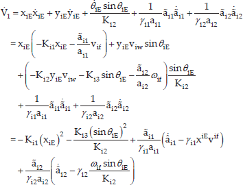
The parameter update laws are chosen as (30) and (31).

${\dot{\widehat{a}}}_{\mathrm{i}1}={\gamma }_{\mathrm{i}1}{\mathrm{x}}_{iE}{\mathrm{v}}_{if}$

(30)

${\dot{\widehat{a}}}_{\mathrm{i}2}={\gamma }_{i2}\frac{{\omega }_{if}\sin {\theta }_{iE}}{K_{i2}}$

(31)

(29) becomes (32).

${\dot{V}}_1=-K_{i1}{\left(x_{iE}\right)}^2-\frac{K_{i3}{\left(\sin {\theta }_{iE}\right)}^2}{K_{i2}}\le 0$

(32)

As t → ∞, E_iq is shown to be a stable equilibrium point. Using Barbalat's lemma, x_iE and θ_iE tend to zero as t → ∞,. Since ã_i1 and ã_i2 are bounded, ẋ_iE and ${\dot{\theta }}_{iE}$ are bounded.

4.2 Adaptive Control of the Dynamic Model

Define the velocity tracking error of the robot R_i as (33).

$E_{ic}={\nu }_i-{\nu }_{ic}=\left[\begin{array}{c}{\nu }_{i1}-{\nu }_{i1c}\\ {\nu }_{i2}-{\nu }_{i2c}\end{array}\right]$

(33)

(7) can be rewritten as (34).

$\bar{M}({\dot{\nu }}_{ic}+{\dot{E}}_{ic})+\bar{V}({\nu }_{ic}+E_{ic})+{\bar{\tau }}_{id}=\bar{B}{\tau }_i$

(34)

Therefore, the differential of E_ic multiply M̄ can be described as

$\begin{array}{l}\bar{M}{\dot{E}}_{ic}=-(\bar{M}{\dot{\nu }}_{ic}+\bar{V}{\nu }_{ic})-\bar{V}{E}_{ic}-{\bar{\tau }}_{id}+\bar{B}{\tau }_i\\ \text{\hspace{0.17em}\hspace{0.17em}\hspace{0.17em}\hspace{0.17em}\hspace{0.17em}\hspace{0.17em}\hspace{0.17em}\hspace{0.17em}\hspace{0.17em}=}-Y_{ic}{P}_i-\bar{V}{E}_{ic}-{\bar{\tau }}_{id}+\bar{B}{\tau }_i\end{array}$

(35)

where M̄V̇_ic + V̄V̇_ic = Y_icP_i and

$Y_{ic}=\left[\begin{array}{ccc}{\dot{\nu }}_{i1c}& {\dot{\nu }}_{i2c}& {\dot{\theta }}_i{\nu }_{i2c}\\ {\dot{\nu }}_{i2c}& {\dot{\nu }}_{i1c}& -{\dot{\theta }}_i{\nu }_{i1c}\end{array}\right],$

$P_i={\left[\begin{array}{ccc}\frac{r_i{}^2}{4b_i{}^2}(m_i{b}_i{}^2+I_i)+I_{iw}& \frac{r_i{}^2}{4b_i{}^2}(m_i{b}_i{}^2-I_i)& \frac{r_i{}^2}{2b_i}{m}_{ic}{d}_i\end{array}\right]}^T.$

Based on [19], the torque controller for the dynamic model is designed as (36).

${\tau }_i={\bar{B}}^{-1}(-K_{id}{E}_{ic}+Y_{ic}{\widehat{P}}_i-u_{is})$

(36)

K_id is a diagonal positive-definite design matrix. P̂_i is the estimate of P_i and P˜_i = P̂_i – P_i. u_is = Asgn(E_ic), where sgn(E_ic) is a sign function and A is a positive-definite controller gain. Define A = ĉ_i0 + ĉ_i1‖v_i‖, ĉ_i0 and ĉ_i1 are the estimate of c_i0 and c_i1 in Assumption 1, and ĉ_i0 = ĉ_i0 – c_i0, ĉ_i1 = ĉ_i1 – c_i1. To design ĉ_i0, ĉ_i1 and P̂, the Lyapunov function is chosen as (37).

$V_2=V_1+\frac{1}{2}{E}_{ic}^T\bar{M}{E}_{ic}+\frac{1}{2}{\stackrel{\sim }{P}}_i^T{\mathrm{\Gamma }}^{-1}{\stackrel{\sim }{P}}_i+\frac{{\stackrel{\sim }{c}}_{i0}^2}{2{\gamma }_{i3}}+\frac{{\stackrel{\sim }{c}}_{i1}^2}{2{\gamma }_{i4}}$

(37)

γ_i3 and γ_i4 are positive constants. The differential of V₂ is denoted as (38).

$\begin{array}{l}{\dot{V}}_2={\dot{V}}_1+E_{ic}^T\bar{M}{\dot{E}}_{ic}^{}+\frac{1}{2}{E}_{ic}^T\dot{\stackrel{̄}{M}}{E}_{ic}^{}+{\stackrel{\sim }{P}}_i^T{\mathrm{\Gamma }}^{-1}{\dot{\stackrel{\sim }{P}}}_i+\frac{{\stackrel{\sim }{c}}_{i0}^{}{\dot{\stackrel{\sim }{c}}}_{i0}^{}}{{\gamma }_{i3}}+\frac{{\stackrel{\sim }{c}}_{i1}^{}{\dot{\stackrel{\sim }{c}}}_{i1}^{}}{{\gamma }_{i4}}\\ \text{\hspace{0.17em}\hspace{0.17em}\hspace{0.17em}\hspace{0.17em}\hspace{0.17em}\hspace{0.17em}=}{\dot{V}}_1+E_{ic}^T\left(-Y_{ic}{P}_i-{\bar{\tau }}_{id}+\bar{B}{\tau }_i\right)+E_{ic}^T\left(\frac{1}{2}\dot{\stackrel{̄}{M}}-\bar{V}\right)E_{ic}^{}+{\stackrel{\sim }{P}}_i^T{\mathrm{\Gamma }}^{-1}{\dot{\stackrel{\sim }{P}}}_i+\frac{{\stackrel{\sim }{c}}_{i0}^{}{\dot{\stackrel{\sim }{c}}}_{i0}^{}}{{\gamma }_{i3}}+\frac{{\stackrel{\sim }{c}}_{i1}^{}{\dot{\stackrel{\sim }{c}}}_{i1}^{}}{{\gamma }_{i4}}\\ \text{\hspace{0.17em}\hspace{0.17em}\hspace{0.17em}\hspace{0.17em}\hspace{0.17em}\hspace{0.17em}=}{\dot{V}}_1+E_{ic}^T\left(Y_{ic}{\stackrel{\sim }{P}}_i-{\bar{\tau }}_{id}-K_{id}{E}_{ic}-A\mathrm{sgn}(E_{ic})\right)+{\stackrel{\sim }{P}}_i^T{\mathrm{\Gamma }}^{-1}{\dot{\stackrel{\sim }{P}}}_i+\frac{{\stackrel{\sim }{c}}_{i0}^{}{\dot{\stackrel{\sim }{c}}}_{i0}^{}}{{\gamma }_{i3}}+\frac{{\stackrel{\sim }{c}}_{i1}^{}{\dot{\stackrel{\sim }{c}}}_{i1}^{}}{{\gamma }_{i4}}\\ \text{\hspace{0.17em}\hspace{0.17em}\hspace{0.17em}\hspace{0.17em}\hspace{0.17em}=}{\dot{V}}_1-E_{ic}^T{K}_{id}{E}_{ic}+{\stackrel{\sim }{P}}_i^T{\mathrm{\Gamma }}^{-1}(\dot{\stackrel{\sim }{P}}+\mathrm{\Gamma }{Y}_{ic}^T{E}_{ic})-E_{ic}^T{\bar{\tau }}_{id}-A{E}_{ic}^T\mathrm{sgn}(E_{ic})+\frac{{\stackrel{\sim }{c}}_{i0}^{}{\dot{\stackrel{\sim }{c}}}_{i0}^{}}{{\gamma }_{i3}}+\frac{{\stackrel{\sim }{c}}_{i1}^{}{\dot{\stackrel{\sim }{c}}}_{i1}^{}}{{\gamma }_{i4}}\end{array}$

(38)

The parameter update laws are selected as (39)-(41).

${\dot{\widehat{P}}}_i=-\mathrm{\Gamma }{Y}_{ic}^T{E}_{ic}$

(39)

${\dot{\widehat{c}}}_{i0}={\gamma }_{i3}\Vert E_{ic}\Vert$

(40)

${\dot{\widehat{c}}}_{i1}={\gamma }_{i4}\Vert {\nu }_i\Vert \Vert E_{ic}\Vert$

(41)

Therefore, (38) can be rewritten as (42).

$\begin{array}{l}{\dot{V}}_2={\dot{V}}_1-E_{ic}^T{K}_{id}{E}_{ic}-E_{ic}^T{\bar{\tau }}_{id}-A{E}_{ic}^T\mathrm{sgn}(E_{ic})+\frac{{\stackrel{\sim }{c}}_{i0}^{}{\dot{\stackrel{\sim }{c}}}_{i0}^{}}{{\alpha }_{i0}}+\frac{{\stackrel{\sim }{c}}_{i1}^{}{\dot{\stackrel{\sim }{c}}}_{i1}^{}}{{\alpha }_{i1}}\\ \le {\dot{V}}_1-E_{ic}^T{K}_{id}{E}_{ic}-\left(A-\Vert {\bar{\tau }}_{id}\Vert \right)\Vert E_{ic}\Vert +\frac{{\stackrel{\sim }{c}}_{i0}^{}{\dot{\stackrel{\sim }{c}}}_{i0}^{}}{{\alpha }_{i0}}+\frac{{\stackrel{\sim }{c}}_{i1}^{}{\dot{\stackrel{\sim }{c}}}_{i1}^{}}{{\alpha }_{i1}}\\ \le {\dot{V}}_1-E_{ic}^T{K}_{id}{E}_{ic}-{\stackrel{\sim }{c}}_{i0}^{}\left(\Vert E_{ic}\Vert -\frac{{\dot{\stackrel{\sim }{c}}}_{i0}^{}}{{\alpha }_{i0}}\right)-{\stackrel{\sim }{c}}_{i1}^{}\left(\Vert {\nu }_i\Vert \Vert E_{ic}\Vert -\frac{{\dot{\stackrel{\sim }{c}}}_{i1}^{}}{{\alpha }_{i1}}\right)\\ \text{\hspace{0.17em}\hspace{0.17em}\hspace{0.17em}\hspace{0.17em}\hspace{0.17em}\hspace{0.17em}=}{\dot{V}}_1-E_{ic}^T{K}_{id}{E}_{ic}\le 0\end{array}$

(42)

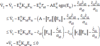
V₂ is non-increasing with time, so it is bounded. Using Barbalat's lemma, x_iE, θ_iE and E_ic tend to zero as t → ∞. θ_iE and θ_iE are bounded. This implies ${\dot{\theta }}_{iE}$ is uniformly continuous. From Barbalat's lemma, ${\dot{\theta }}_{iE}\to 0$ as t → ∞. According to (23), (24) and (33), variable ${\dot{\theta }}_{iE}$ can be described by the equationK_iy v_iw y_iE → 0. v_iw is a bounded function of time. These imply that y_iE has to converge to zero. As t → ∞, E_iq = 0 is an asymptotically stable point. Therefore, the error E = (E^T_iq E^T_ic)^T = 0 is an asymptotically stable equilibrium point.

5. Simulation Results

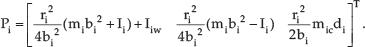
In this section, the physical parameters of the robots are as b_i = 0.125m, d_i = 0.15m, r_i = 0.08m, m_ic =4kg, m_iw = 1kg, I_ic = 2.325 kgm², I_iw = 0.005 kgm² and I_im = 0.0025. The parameters for the adaptive controllers are chosen as K_i1 =0.1, K_i2 =0.2, K_i3 = 0.28, K_id = diag{0.5,0.5}, γ_i1 = γ_i2 = 0.001, γ_i3 = γ_i4 = 0.01 and Γ = diag{0.01,0.01, 0.01}.

5.1 First Simulation

Fig. 7 shows the trajectories of three robots forming a line formation at t=2.9s, t=3.3s, t=3.7s and t=6.0s. The desired distance of follower robots 1 and 2 with the leader robot are equal to l₁₀ = 0.9m and l₂₀ = 0.45m, respectively. The desired bearing angles are β₁₀ = β₂₀ = 0. The protected shell radius of the follower robots are 0.16m. The initial state of the leader robot, follower robot 1 and follower robot 2 are as (0.5,1.5,0)^T, (-0.65,2.5,0)^T and (-0.65,0.5,0)^T, respectively. The leader robot's trajectory is defined as

Figure 7.

The trajectories of three robots avoiding collision based on the static collision priorities of two follower robots. (a) t=2.9s, (b) t=3.3, (c) t=3.7, (d) t=6.0s

$x^L=0.4t+0.5$

(43)

$y^L=1.5$

(44)

Based on the collision priority process, the two follower robots' static priorities are not the same so that the follower robot is selected to execute the collision avoidance algorithm by the static priorities comparison result. Follower robot 1's static priority is smaller than follower robot 2's. Therefore, follower robot 1 avoids the collision with follower robot 2 using the collision avoidance algorithm, while follower robot 2 keeps tracking the formation.

Along the trajectories in Fig. 7(d), the trajectory and velocity tracking errors of follower robots 1 and 2 are shown in Figs. 8–11. The simulation was run 50 times to take average values and input noise is|τ_id | ≤ 3. From the results, the trajectory and velocity tracking errors approach to zero.

Figure 8.

The trajectory errors of follower robot 1

Figure 9.

The trajectory errors of follower robot 2

Figure 10.

The velocity errors of follower robot 1

Figure 11.

The velocity errors of follower robot 2

To better show the performance of the static priority strategy in reducing the collision path and in solving the deadlock problem, Fig. 12 is compared with Fig. 7 (d). In Fig. 12, two follower robots track the same leader robot as in Fig. 7 (d), without the static priority comparison result. This means that follower robot 2 must avoid collision using the collision avoidance algorithm, and follower robot 1 keeps tracking the formation trajectory, when the collision danger occurs. As seen from Fig. 12, follower robot 2 cannot reform the formation with the leader robot. Therefore, the static priority strategy is essential to reduce the collision path and solve the deadlock problem.

Figure 12.

The trajectories of three robots avoiding collision without the static priority comparison result

5.2 Second Simulation

Fig. 13 shows three robots' trajectories forming a triangle formation at t=2.7s, t=3s, t=3.5s, t=5s and t=10s. The desired distance of follower robots 1 and 2 with the leader robot are equal to l₁₀ = l₂₀ = 0.45m, and the desired bearing angle are β₁₀ =-∂/4 and β₂₀ = ∂/4, respectively. The protected shell radius of follower robots 1 and 2 are 0.16m, 0.16m, respectively. The initial state of the leader robot, and follower robots 1 and 2 are as (0.5,1.5,0)^T, (-0.65,2.5,0)^T and (-0.65,0.5,0)^T, respectively. The leader robot's trajectory is defined as (43) and(44).

Figure 13.

The trajectories of three robots avoiding collision based on the dynamic collision priorities of two follower robots. (a) t=2.7s, (b) t=3s, (c) t=3.5s, (d) t=5s, (e) t=10.0s

In this case, because the two follower robots' static priorities are the same, the selection for the follower robot to do the collision avoidance algorithm is based on the dynamic priority comparison result. Due to the smaller dynamic priority, follower robot 1 is required to avoid the collision with follower robot 2.

For the trajectories in Fig. 13(e), the trajectory and velocity tracking errors of follower robots 1 and 2 are shown in Figs. 14–17. The simulation was run 50 times to take average values and input noise is |τ_id | ≤ 3. The trajectory and velocity tracking errors approach to zero clearly.

Figure 14.

The trajectory errors of follower robot 1

Figure 15.

The trajectory errors of follower robot 2

Figure 16.

The velocity errors of follower robot 1

Figure 17.

The velocity errors of follower robot 2

Comparing with Fig. 13 (e), Fig. 18 shows that the three robots track the same trajectories as in Fig. 13 (e), without the dynamic comparison result. When collision danger happens, follower robot 2 must avoid collision using the collision avoidance algorithm, and follower robot 1 keeps tracking the formation trajectory. Table 2 shows the performance of the dynamic priority strategy in minimising the turning angle of the follower robot more clearly.

Figure 18.

The trajectories of three robots avoiding collision without the dynamic priority comparison result

Table 2 demonstrates the incremental collision path length and turning angle during forming and maintaining of the formation in Fig. 13 (e) and Fig. 18.

Table 2.

The comparison results of incremental collision path length and turning angle during forming and maintaining the formation within and without priority comparison results.

Collision avoidance	Incremental path length (metres)		Incremental turning angle (rad)
	FR1	FR2	FR1	FR2
within the priority comparison result	3.3299	x	1.9769	x
without the priority comparison result	x	6.7401	x	5.1945

Using the dynamic priority strategy, the incremental collision path length in Fig. 13 (e) is shorter than the incremental collision path length in Fig. 18, and the turning angle in Fig. 13 (e) is quite substantially minimized.

5.3 Third Simulation

The third simulation demonstrates that a large team of robots can benefit from the proposed collision avoidance methods. In Fig. 19, the desired distances of the four follower robots with the leader robot are equal to l₁₀ = 0.85m and l₂₀ = 0.45m, l₃₀ = 0.4m, l₄₀ = 0.4m, respectively. The desired bearing angles are β₁₀ = β₂₀ = 0, β₃₀ = ∂ / 4 and β₄₀ = -∂ / 4. The protected shell radius of the follower robots are 0.16m. The initial state of the leader robot and follower robots 1–4 are designed as(0.5,1.5,0)^T, (-0.55,2.5,0)^T, (-0.55,0.5,0)^T, (-0.6,2,0)^T and (-0.6,1,0)^T, respectively. The leader robot's trajectory is defined as (45) and (46). The collision danger firstly takes place between follower robot 3 and follower robot 4. Based on the dynamic priority strategy, follower robot 3 does the collision avoidance algorithm. Follower robot 2 and follower robot 3 must secondly solve the collision avoidance problem. According to the static priority strategy, follower robot 2 is required to do the collision avoidance algorithm. Finally, follower robots 1 and 2 must take the collision avoidance into consideration. Based on the static priority strategy, follower robot 1 avoids the collision.

$x^L=0.55t+0.5$

(45)

$y^L=1.5$

(46)

The trajectory errors of the follower robots 1–4 with the trajectories in Fig. 19 are shown in Figs. 20–23. From the results, the trajectory errors stably converge to zero.

Figure 19.

The trajectories of five robots avoiding collision based on four collision avoidance processes

Figure 20.

The trajectory errors of follower robot 1

Figure 21.

The trajectory errors of follower robot 2

Figure 22.

The trajectory errors of follower robot 3

Figure 23.

The trajectory errors of follower robot 4

The velocity errors of follower robots 1–4 with the trajectories in Fig. 19 are shown in Figs. 24–27. From the results, the velocity errors approach to zero.

Figure 24.

The velocity errors of follower robot 1

Figure 25.

The velocity errors of follower robot 2

Figure 26.

The velocity errors of follower robot 3

Figure 27.

The velocity errors of follower robot 4

5.4 Fourth Simulation

To show the validation of the adaptive controllers, the fourth simulation presents a large group of robots forming and maintaining formation avoiding collisions in sinusoid trajectories. In Fig. 28, the desired distances of the four follower robots with the leader robot are equal to l₁₀ = 1.2m and l₂₀ = 0.6m, l₃₀ = l₄₀ = 0.8m, respectively. The desired bearing angles are β₁₀ = β₂₀ = ∂ / 4, β₃₀ = -∂ / 6 and β₄₀ = -∂ / 2. The protected shell radius of the follower robots are 0.16m. The initial state of the leader robot and the follower robots are given by (0,0,0)^T, (-1.2,-1.2,0)^T, (-0.8,-1.7,∂/6)^T, (-0.9,0.6, ∂/6)^T and (-0.8,0.3,0)^T, respectively. The leader robot's predefined trajectory is denoted as (47) and (48). Based on the static priority strategy, follower robot 1 avoids the collision with follower robot 2. In addition, follower robot 3 is required to avoid collision with follower robot 4 by using the dynamic priority strategy.

$x^L=0.35t$

(47)

$y^L=1.5\sin (0.15t)$

(48)

The trajectory errors of follower robots 1–4 with the trajectories in Fig. 28 are shown in Figs. 29–32. From the results, the trajectory errors stably converge to zero.

Figure 28.

The trajectories of five robots avoiding collision based on four collision avoidance processes

Figure 29.

The trajectory errors of follower robot 1

Figure 30.

The trajectory errors of follower robot 2

Figure 31.

The trajectory errors of follower robot 3

Figure 32.

The trajectory errors of follower robot 4

The velocity errors of follower robots 1–4 with the trajectories in Fig. 28 are shown in Figs. 33–36. From the results, the velocity errors approach to zero.

Figure 33.

The velocity errors of follower robot 1

Figure 34.

The velocity errors of follower robot 2

Figure 35.

The velocity errors of follower robot 3

Figure 36.

The velocity errors of follower robot 4

6. Experimental Results

6.1 The Robot Platform

The positions and attitudes of the three nonholonomic robots as shown in Fig. 37 are measured using a CCD camera (640×480) on the ceiling. In addition, the diameter of each wheel is 4.3 cm, and the distance between the left and right wheels is 6.9cm. The weight of the robot is 0.4kg.

Figure 37.

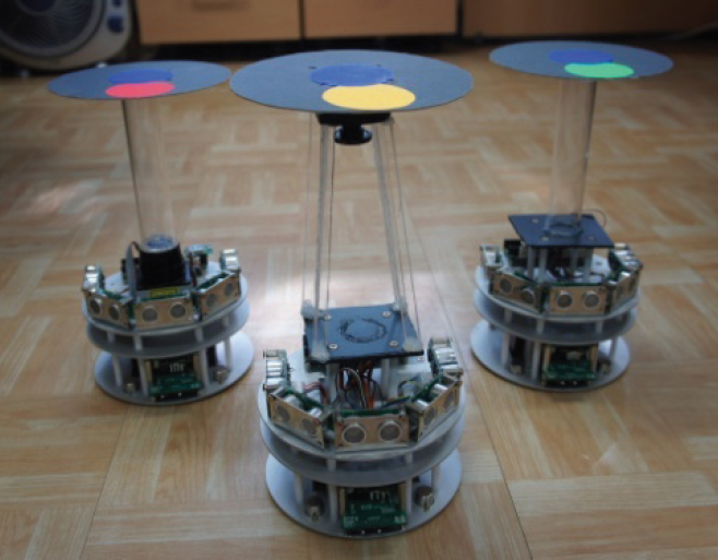
Three nonholonomic robots in the experiment

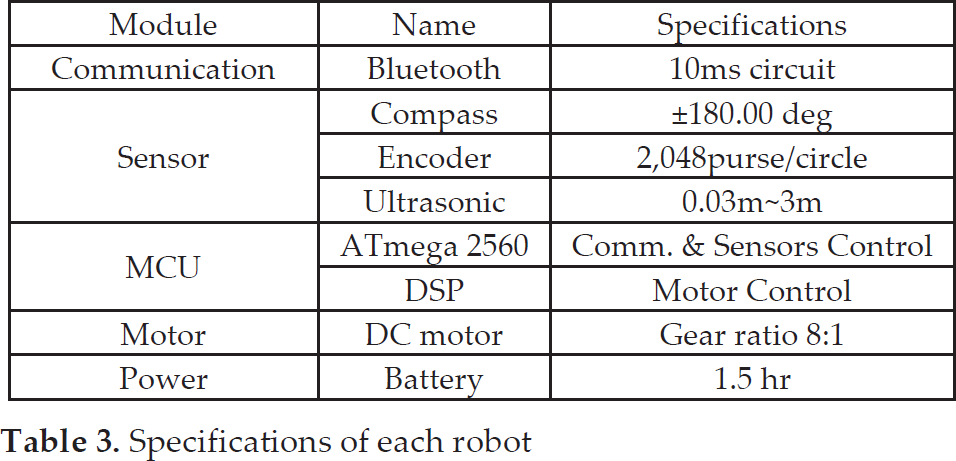
Each robot is equipped with five modules, including communication module, sensor module, MCU module, motor module and power module. The specifications of the modules are shown in Table 3.

Table 3.

Specifications of each robot

Module	Name	Specifications
Communication	Bluetooth	10ms circuit
Sensor	Compass	±180.00 deg
	Encoder	2,048purse/circle
	Ultrasonic	0.03m∼3m
MCU	ATmega 2560	Comm. & Sensors Control
	DSP	Motor Control
Motor	DC motor	Gear ratio 8:1
Power	Battery	1.5 hr

6.2 The System Implementation

The information of the leader robot, such as encoder values and compass sensor value, is sent to server PC by Bluetooth.

As shown in Fig. 38, the following steps are the executions for the follower robot to track the leader robot while avoiding collisions. (1) Based on the ultrasonic sensor values, if both of the follower robots are close enough, they send the collision flag to the server PC. (2) When the server PC receives a collision flag, it calculates the waypoint based on the four collision avoidance processes. Otherwise, the waypoint is calculated using the leader robot's information. (3) The server PC calculates torques and sends motor commands to the follower robot by Bluetooth. (4) The follower robot drives the DC motors based on the control law. (5) The follower robot transmits encoder values and the angle value to the server PC. (6) Based on the encoder values and the angle value, a localization process is performed on the PC. (7) The states of the follower robots are changed according to the adaptive controllers. In Fig. 38, the processes inside the dash block are executed in the PC, while the other blocks are processed by the onboard modules of the follower robots.

Figure 38.

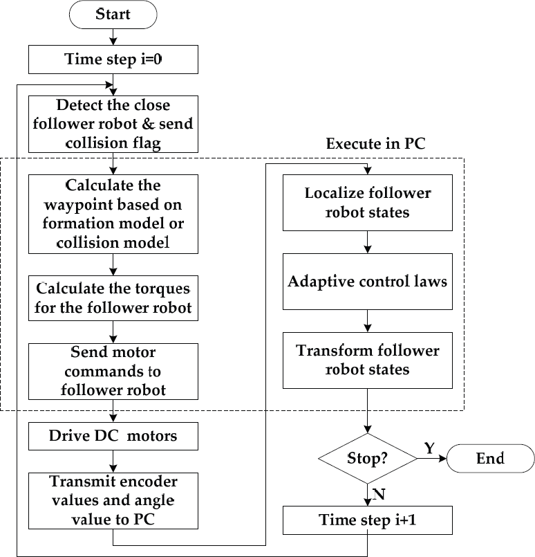
The overview of the system implementation for each follower robot

6.3 Experiment

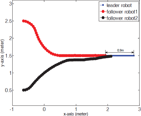
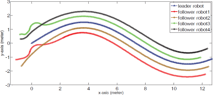
In the experiment, three robots are executed to form and maintain a line formation, while avoiding collisions between follower robots. The radius of the protected shell of each robot is 8cm. The other parameters for the adaptive controllers are chosen as K_i1 = 0.1, K_i2 = 0.2, K_i3 = 0.28, K_id = diag{0.5,0.5}, γ_i1 = γ₂ = 0.001, γ_i3 = γ_i4 = 0.01 and Γ = diag{0.01,0.01,0.01}. The initial states of the leader robot and follower robots 1 and 2 are (26cm,15cm,0)^T, (0,0,0)^T and (0,30cm,15deg)^T, respectively. The desired distances for follower robots 1 and 2 with the leader robot are defined as l₁₀ = 60cm and l₂₀ =30cm, respectively. The desired angles of the follower robots are β₁₀ = β₂₀ = 0. Fig. 39 shows the trajectories of the three robots forming and maintaining a line formation. Based on collision priority strategy and the collision avoidance algorithm, when two follower robots form the formation, follower robot 1 avoids the collision with follower robot 2.

Figure 39.

The formation tracking trajectories of the three robots while avoiding collision

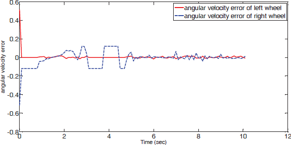
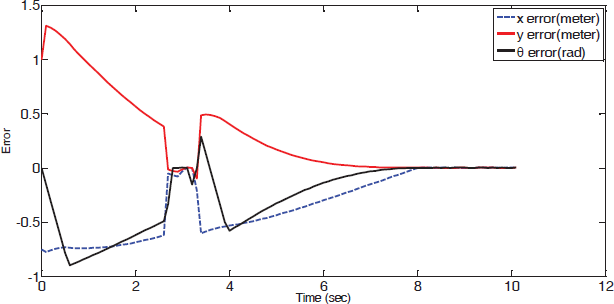
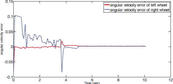
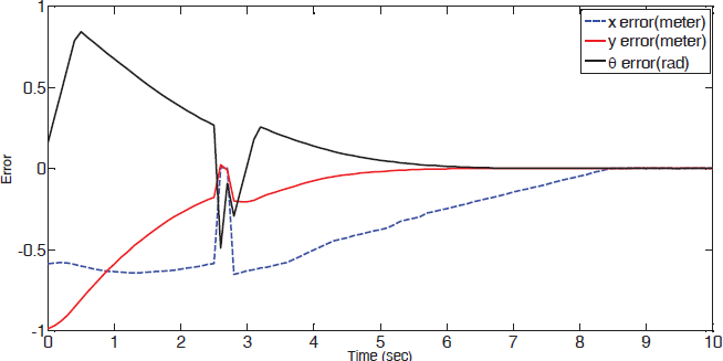
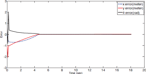
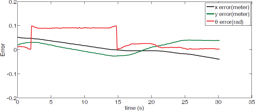
The state errors of follower robots 1 and 2 are shown in Figs. 40 and 41. In Fig. 40, when follower robot 1 avoids the collision, there is an angle error which is reduced after avoiding collision.

Figure 40.

The state errors of follower robot 1

Figure 41.

The state errors of follower robot 2

Video snapshots are presented in Fig. 42, where three robots form a line formation while avoiding collision.

Figure 42.

Snapshot of three robots forming a line formation and avoiding collision between the follower robots: (a)t=0s, (b)t=3s, (c)t=5s, (d)t=10s, (e)t=16s, (f)t=20s, (g),t=24s (h),t=30s (right, then down).

7. Conclusions

In this paper, the proposed four collision avoidance processes were used to generate collision-free trajectories for nonholonomic mobile robots when forming and maintaining formation. In order to minimize the turning angle of the robot, solve the dead-lock problem and find the shortest collision avoidance path, the collision priority strategy was coordinated with the collision avoidance algorithm. The adaptive control algorithm, based on Lyapunov analysis, is designed for the trajectory and velocity tracking errors of each robot to converge to zero. Finally, the simulation and experiment results demonstrate the effectiveness of the proposed methods.