Sage Journals: Discover world-class research

Abstract

Localizationis of vital importance for an unmanned vehicle to drive on the road. Most of the existing algorithms are based on laser range finders, inertial equipment, artificial landmarks, distributing sensors or global positioning system(GPS) information. Currently, the problem of localization with vision information is most concerned. However, vision-based localization techniquesare still unavailable for practical applications. In this paper, we present a vision-based sequential probability localization method. This method uses the surface information of the roadside to locate the vehicle, especially in the situation where GPS information is unavailable. It is composed of two step, first, in a recording stage, we construct a ground truthmap with the appearance of the roadside environment. Then in an on-line stage, we use a sequential matching approach to localize the vehicle. In the experiment, we use two independent cameras to observe the environment, one is left-orientated and the other is right. SIFT features and Daisy features are used to represent for the visual appearance of the environment. The experiment results show that the proposed method could locate the vehicle in a complicated, large environment with high reliability.

Keywords

Visual Appearance Sequential Localization Feature Matching Unmanned Vehicle

1. Introduction

Before an unmanned vehicle decides where to drive, it should know where it is. So the problem of localization becomes very important, and it has also received much attention. The most popular localization approach is using a GPS receiver [1,2]. A real-time dynamic differential GPS could locate a vehicle accurately with a precisionofone-centimetre if enough information from several satellites is available. Unfortunately, in some areas such as dense urban environments, buildings, thick trees or tunnels may mask the information from the satellites, rendering the GPS information discontinuous. Xu [3] applies a Kalman filter-based model for effectively correcting GPS errors in map matching, which could handle the biased error and the random error of the GPS signals. However, the GPS sensor alone is not enough for the vehicle system to locate itself and inertial equipment are used to compensate the drawback of the GPS system [4]. Additionally, some other sensors such as laser range finders and distributed sensors are used to locate the mobile system. But the nature of the environment always contains much more information in the appearance, so the visual information is more and more relevant, which is still a challenging problem.

In this paper, we focus on the problem of recognizing locations by visual appearance information. Vision-based localization methods typically need the camera intrinsic parameters (focal length, optical centre and distortion) and extrinsic parameters (robot-relative pose), which have to be determined in advance and cannot change over time. With these parameters, we can construct the exact geometric structure of the environment and the sensors' positions. This is also known as Structure From Motion (SFM) or Simultaneously Localization and Mapping (SLAM). Usually, a camera calibration process is needed in advance, which is time consuming for real-time applications, however, on-line calibration is also still a challenging problem. Moreover, it is difficult to maintain the parameters as unchanged for a long time.

In particular, we consider using a known map to locate the vehicle with uncalibrated cameras, and propose a vision appearance-based sequential localization algorithm. In our application, we use two side-orientated cameras on the vehicle to recognize the current location of the system. The reason for using two side-orientated cameras is that when we drive on a road, it is very hard to recognize where we are by using only the frontal information. Therefore, the diagonal camera will offer a big visual field with much more visual information. In the proposed method, first, we drive the vehicle around the environment and keep the visual appearance of the roadside and the locations to where the vehicle can obtain the information. We carefully choose the most distinctive and invariable image to form a visual representation of the environment, e.g., a visual map. Second, when the vehicle visits the place again, we match the newly captured images to the known map sequence, and then the unmanned vehicle could know where it is. So if the vehicle drives on the same road, it could locate itself from the roadside appearance automatically, and guide the vehicle where to go [5]. We have tried two image representation methods in our system, the SIFT feature-based method [6] and the Daisy feature-based method[7].

We found that the SIFT feature-based method could get a more reliable and faster result. Our unmanned vehicle is shown in Figure 1, driving around our campus. We can use the proposed method to guide the Spring-Robot to drive in a large-scale environment. The rest of the paper is organized as follows: section 2 is a brief overview of related works. In section 3, we present the sequential matching algorithm. Then the experimental results of the proposed method are presented in section 4. Finally, we present conclusions and the discussion of future work in section 5.

Figure 1.

The Spring-Robot, equipped with laser, GPS, cameras and some other sensors. The orientation of the left camera is 45 degrees left, and the right camera is 45degrees right, which are used in our application. Now it is driving around our campus, where the environment beside the road is very complicated. The GPS signal is badly affected by the buildings and the thick trees.

2. Related Work

The problem of localization and navigation, which is a fundamental component of an unmanned vehicle system to drive on the road, is closely related to the problem of Structure Form Motion (SFM). Significant advances have been made in SFM in recent years, and many vision-based approaches have been proposed to deal with this problem. These approaches contain two main classes with respect to whether or not they use prior knowledge of the environment.

In one class, only the initial location is given. Then probabilistic reasoning algorithms are used to track the robot location. One outstanding example of this class is the visual odometry method [8], in which the front-end is a point-based tracker. Point features are matched between pairs of consecutive frames and linked into trajectories at video rate. Robust estimation of the camera motion is then produced from the feature tracks using a geometric hypothesis and test architecture. It is very useful to estimate the motion of a mobile system, but the system does not keep a map of the environment, and it cannot recognize the same location when it travels back from a long distance. A Kalman filter-based SLAM method is proposed in [9], which can reconstruct an environment of a small space by using a set of sparse point features and track the camera's pose and position precisely. However, the poor stability and the cubic increasing computational complexity stop it from being applied on a real mobile vehicle system. In order to increase the stability of a SLAM system, improvements have been made in many aspects such as FastSLAM with SIFT descriptor [10], where the SIFT feature is used to increase the robustness of feature matching. Eade and Drummond [11] apply a FastSLAM-type particle filter to a single camera SLAM, which has a computational cost linear with the number of the visual landmarks, but it is still difficult to use on a mobile vehicle system in practice. A more practical method has been recently presented in [12,13]. The visual SLAM and visual odometry are combined together to build a dense 3D map of the environment, which is very useful for autonomous vehicle navigation, path planning, obstacle avoidance, etc.

In the other class, the visual map of the environment is known in advance. Thus distinctive representation of the environment is of vital importance to the reliability of the localization result. Klein [14] uses key-frames to represent the environment for a SLAM system. Paul [15] uses salient features to increase the distinction of the visual landmarks. Williams [16] uses the random tree method to choose the most distinctive point features. These approaches give impressive real-time performances in small environments and are practical in very smallenvironments. In very large environments however, GPS information is required to provide the ground truth.

Except for the above, there are several works very close to ours which investigate the problem of autonomously driving in an open and complex environment on a very large scale using only visual appearance information. Koch [17] use a set of SIFT features to represent the place and construct a topological map of the indoor environment. Together with a collision avoidance system, they could navigate the robot safely and reliably through the environment. Ho[18] encodes the similarity between all possible pairs of scenes in a “similarity matrix”, and thentreats the loop-closing problem as the task of extracting statistically significant sequences of similar scenes from this matrix. With the help of GPS ground truth information, it can work in a very large environment. Mark [19] uses a probabilistic approach to the problem of robot localization and mapping. They use bag-of-words with SURF features to represent the visual appearance of the current place and a Chow-Liu tree is constructed to capture the co-occurrence statistics of the visual words, then a Bayes probabilistic approach is used to determine whether the observed place is old or new. With GPS, it can construct a SURF feature words-based map on a very large scale. When the robot returns, it can recognize whether or not it has been to this place. We use a set of SIFT features to represent the visual appearances of the environment. The map frames are grouped together with respect to their similarity and the statistically significant sequences of similar scenes are used to locate the vehicle. We drive it in a more simple but practical way. More details can be found in the following sections.

3. Sequential Probability Localization

Our visual appearance-based localization method consists of two phases: recording phrase and matching phrase. In the recording phase, a visual map of the environment is constructed. It contains a sequence of locations and each location is represented by point features of its visual appearance. In the matching phase, the vehicle drives on the road with the guidance of the map. The algorithm are shown as follows:

Sequential Vision Localization Algorithm

1. record a map sequence,

M = {l_{1}, l_{2} \dots l_{n}}

2. describe the map frame, the i_th map frame representation

l_{i} = {f_{p}^{i}}_{p = 1 \dots p}

3. observe the environment on-line, the current view representation

y_{t} = {f_{q}^{t}}_{q = 1 \dots Q}

4. match the observation with the map sequence, if initial location is known

l_{t + 1} = \underset{l^{*} \in M^{*}}{\arg \max} {P (l^{*} | M^{*}, y_{t + 1}, u_{t})}

or else do

l_{g} = l \in M & P_{t} > t h r e s h o l d

until we get unique successive matches

5. guide the vehicle.

3.1 Probability Analysis

After the recording step, we get a visual map of the environment, represented as M {l₁,l₂···l_n}. l_n is the visual appearance representation of location n. At time t, the location of vehicle is l_t, the current observations from the cameras are y_t, the system input is u_t. Then we can get the current location of the vehicle from Equation(1),

P (l_{t + 1} | y_{1 : t + 1}, M, u_{1 : t}, l_{1 : t}) \overset{m a r k o v}{=} P (l_{t + 1} | y_{t + 1}, M, u_{t}, l_{t})

(1)

More information about this can be found in chapter 7 in [20]. In order to locate the vehicle, we have to calculate the joint probability distribution when each observation arrives. It is a time consuming job because of its high dimensions, but we find that the process is Markov, as is shown in Equation (1). With a known velocity and a sequential map, the problem can be simplified. When we get a new observation y_t+1 after we pass location l_t, we can localize the vehicle by searching a few nearby map frames. This is because the map is composed of a keyframe sequence that is locally distinctive, and the vehicle drives under the same sequence order as the map. So we do not have to calculate the probability distribution of the vehicle in the whole map, only the vicinity map sequence M* concerned. This can be shown as the following function,

l_{t + 1} \overset{​}{=} \underset{l^{*} \in M^{*}}{argmax} {P (l^{*} | M^{*}, y_{t + 1}, u_{t})}

(2)

The information of l_t in Equation (1) is used to define M*in Equation (2). But if we do not know the initial location or l_t, a global localization method will be needed. With one successful matching it is hard to give the right location because the maps are not globally distinctive from each other. So several observations are needed to determine the current location. The mathematical description of this problem is to get P_t = P(l_t|y_i:t,M,u_i:t). This function can be translated into a more practical function (3). One observation will give m potential locations l_g1 = {l_{g1_1},l_{g1_ 2}···l_{g1_m}}. Doing this several times, we can get a unique location sequence l_p = {l_{g1_ i},l_{g2_ j}···}. When we get a unique successive match _g ₁ we can get the right location, see Figure 4. More practical instructions are given in section 3.4.

l_{g} = l \in M & P_{t} > t h r e s h o l d

(3)

3.2 Key-frame Selection

The visual map of the environment is constructed in the recording step. The image sequence is collected by the left and the right cameras when the vehicle is driven through the environment. We choose images as key-frames under several rules: (1) whether the image is distinctive to its vicinity frame images, (2) whether the visual appearance of the location can remain unchanged for a long time, (3) whether the location is human sensitive. It is not very difficult to select locally distinctive frames automatically [21]. We match the vicinity images with each other and select the more informative which contain more point features than a certain number, and less matched images as key-frames. Human sensitive images are harder to select automatically as they generally need the assistance of a human. They are also unnecessary for a vehicle to localize itself, although they can give us humans a sense of knowledge that is very useful to human-robot interaction. So we apply this rule in the case that there are a few images, which are close and distinctive to each other, we choose the most human sensitive image as the map sequence. The third rule is difficult for machines, so we carefully delete some distinctive images with temporary visual appearance, such as cars, a crowd of people and so.

Figure 2 shows some selected key-frames in our map sequence, we can see that under our rules, locations such as buildings, crossings and gates are most prone to be selected. Most of them are human sensitive that can benefit from human-robot interaction. We also find that in some locations, the views almost do not change over a long distance, but in others, the views may change quickly. So the distances between the key-frames vary a great deal. Only one frame is selected for one location in our algorithm. This is because firstly, the map frame should be locally distinctive; secondly, in the on-line phase, the vehicle only drives a slightly different path to the explored path and therefore the view will not change much.

Figure 2.

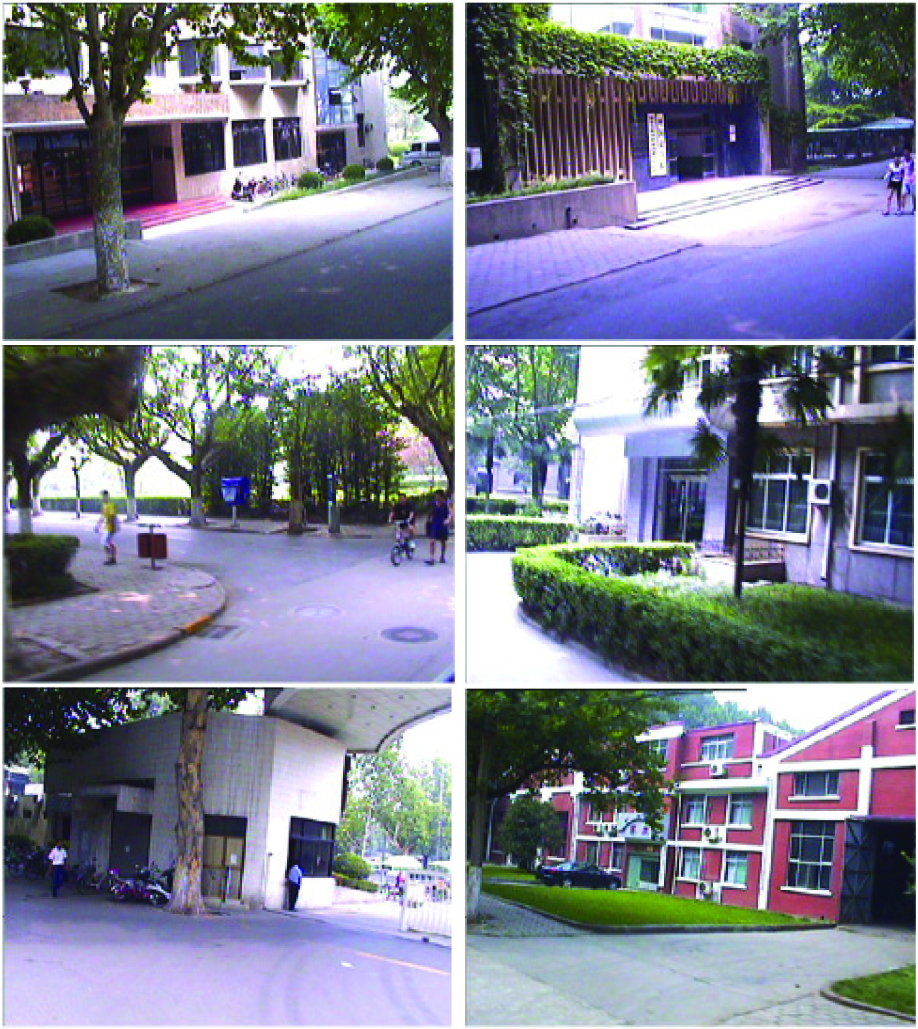
Samples of the selected key-frames with known ground truth locations, which are used as the map sequence of the environment. They are collected by the vehicle running on the road in the exploring phase. The left column is from the left-orientated camera and the right column is from the right camera.

3.3 Map Representation

The map is constructed using a sequence of key-frames with ground truth locations. Each key-frame is represented by a collection of SIFT features. The points are locally extreme in the scale space and each feature is endowed with a 128 dimension descriptor, which captures the orientation information of the local image region centred at the key point. The SIFT feature is rotationally invariant and robust with respect to large variations in viewpoint and scale. But in order to get a more precise location, we do not match them in large scale, so the scale space is limited here. This could also benefit the processing speed.

In the experiment, we found that most selected frames are building appearances, and we also found that more corner features could be obtained in the images with buildings. So we apply another kind of feature, the Harris corner [22], which is scale invariant to some extent and can be computed quickly. Then we use the Daisy descriptor to represent the features in the image. The Daisy descriptor is primarily used to deal with a dense matching problem, which uses200-dimension information to represent a key-point. The Daisy descriptor is similar to the SIFT descriptor. The difference between the SIFT descriptor and the Daisy descriptor is that SIFT calculates the gradient information in a statistical way, while Daisy does it by filtering, thus it is supposed to work faster than the SIFT descriptor.

The map frames are locally distinctive, but they are not globally unique. So when we construct the map, similar images are grouped together like the similar matrix in [18]. One of them is selected as their common representation. This can largely decrease the computational cost, especially in a very large environment where there are thousands of key-frames.

3.4 Sequential Matching

The second part of our approach is the sequential image matching, as shown in Figure 3. The selected key-frames are represented with a connection of key-points. If the initial location is known, we can get the locations of the vehicle on-line by matching the new visual observation periodically to the vicinity key-frames. When we capture an image, we will extract the key-point features, and construct a kd-tree with them. Then we drop the features of the vicinity map frames into the tree. If we find a best matching, we will know that the vehicle is near the location of the corresponding map frame, and mileage information can be used to help choose the potential matching map sequence.

Figure 3.

Match the on-line observation to the map sequence. The solid lines show successful matches, the dash lines represent the potential matching places.

Suppose at time t, P features are detected, y_t = {f^t_p}_p=1···p, f^t_p represents the p_th feature in the t_th frame. Then a kd-tree is constructed, the similarity between features is

d = ∥ f_{p}^{t} - f_{p}^{i} ∥

(4)

where f_pⁱ represents the q_th feature in the i_th map frame. If f ⁱ _p , the two points are considered as matched, where s is a point feature matching threshold. The current observed images are matched with each of the vicinity map images. The number of the matched features between the current observation and the map frames are used to judge whether or not they are matched. The map frames, which give the biggest number of matched features and while bigger than a certain threshold, are considered as matched images. This is the practice of Equation (2).

If the initial position is unknown, the global location method in section 3.1 will be activated. The image matching method is the same as above. As can be seen from Figure 4, for each observation will be matched with all the map frames, and all the good matchesare selected. Good matches are judged by the number of the matched features. More details are shown in the experiment. Do this several times until a successive match appears.

Figure 4.

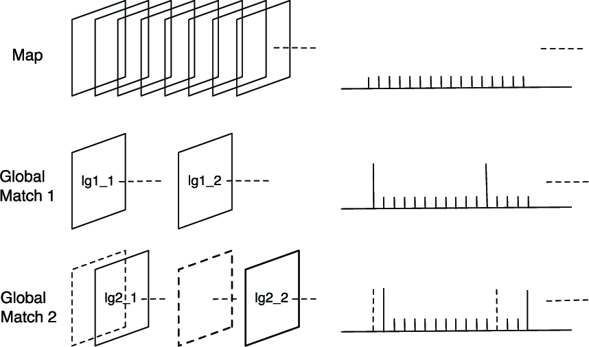
Global localization. The first line is the map sequence and the vehicle locations. The followings are the matched observations. If a map frame is observed, it will give some location suggestions for the vehicle, which are the longer vertical lines on the right of this figure. After several global matches, we can get a unique success match. For example, l_g_{1_1} and l_g_{2_1} are the only two successive matches, so we can tell that the vehicle is at l_g_{2_1} after global match 2.

3.5 Visual Navigation

Except for unmanned vehicle localization, our system could also be used for navigation. It can guide the vehicle where to go, especially when the vehicle encounters a corner or a cross, the map sequence will branch. By giving a certain destination in the map, the system can tell the vehicle which branch sequence of the map to follow, and prepare for a turning in advance. Similar to [17], our localization method could also be used to navigate in indoor environments. If it integrates with an obstacle avoidance system, it can also guide the vehicle drive in a gallery automatically.

4. Experiment Result

In the experiment, both the SIFT descriptor and the Daisy descriptor are tested to locate the unmanned vehicle in a large-scale environment. The Spring-Robot drives at 4m/s around our campus. The cameras are left- and right-orientated. Each has a field of 40×30 degrees with a 320×240 pixels resolution. The camera works at a rate of 10 Hz. The computer is equipped with an Intel Core2 Duo CPU E6550 @ 2.33 GHz with 2 GB memory. We obtain more than 5000 frames on the campus, but it is not necessary to gain the global position in every single frame in this application, and also, considering the computational complexity, we only deal with the observations every five frames. In the experiment, 84 locally distinctive places with ground truth locations are selected to construct the visual map.

The sequential locations of the selected key-frame have a distance of about 5 metres to 30 metres because of the local distinctive rule. Consider that the new observation could only be matched when the vehicle moves to the places that are slightly different from the locations where the key-frames are collected. So the vehicle location precision varies accordingly, from a few metres in the places with dense key-frames to more than 20 metres in the places with spare key-frames.

First we test the sequential localization matching method. In this application, the scale is limited to a small number when we extract the SIFT features. Each feature is described by a 128-dimension vector. For a 320×240 image, the region of interest is set to [10,30,300,140], which are left, top, right and bottom of the image. This is because that in this application, the top of the image is mainly leaf and the bottom is mainly ground, which do not contain much useful information. The feature calculation and the image matching processes are managed in different CPU cores. Considering the correct matching ratio and the calculation time, only five vicinity map frames are used to match with the current observation. In this situation, the critical time process is the calculation of the feature detection and description.

As is well-known, the Harris corner is computationally low cost and very robust to light and scale. The Daisy descriptor, which is very close to the SIFT descriptor, can be computed much more efficiently than the SIFT descriptor. So we use the Harris corner with Daisy descriptors to represent the images. The experiment conditions are the same as when we use the SIFT features. The resultscan be seen in Table 1. But unfortunately, this feature shows no remarkable advantage over the SIFT feature in this application. Considering the trade-off between the computational time and matching ratio, we use the SIFT features on the images with a resolution of 256×192 in the application.

Table 1.

In the experiment, the image resolution is very important, so we tested several frame sequences with different resolutions. We tried to maintain the wrong localization rates at around 1 percent and with no tracking lost. This time we could not get a real-time result, but we were not very far from this. With a left-orientatedcamera and a right-orientated camera, we could get a higher localization ratio, which is also more reliable.

Feature type		Average Feature Number	Feature Calculation Time (ms)	Matching Time (ms)	Location Recognizing Rate			Wrong Matching (%)
Feature type		Average Feature Number	Feature Calculation Time (ms)	Matching Time (ms)	Left	Right	Total	Wrong Matching (%)
SIFT	320×240	128	360	317	0.88	0.94	0.97	1.35
	256×192	76	221	145	0.82	0.88	0.90	1.36
	160×120	31	89	48	0.49	0.54	0.73	1.26
Daisy	320×240	158	247	309	0.63	0.78	0.90	1.28
	256×192	121	199	299	0.42	0.69	0.79	1.40

From Figure 5 we can see that as the number of features increases, the feature detection and description time increases, but the matching ratio decreases. We may assume that fewer features could get better results, but as Table 1 shows, the map recognition rate decreases as the number of features decreases, in other words, more features could get more reliable matching results. Thus, the match ratio should not be used as the matching threshold. We use the absolute number of matched features to judge whether or not the two images are similar.

Figure 5.

The relationship between the feature number and the calculation time (red and blue lines). As the number of features increases, the computation time increases. The green line shows the relationship between the feature number and the feature match ratio.

The matching results of the frames observed from the right and the left cameras is shown in Figure 7. The two cameras could compensate each other to gain a higher matching ratio than anyone of them - Table 1 gives the numeric results. Figure 6 shows the changing of the calculation time and the feature number in the on-line experiment. The proposed method could get an almost constant time result. It cannot work in real-time currently, but we are notvery far from this.

Figure 6.

The SIFT feature based approach with an image resolution of 256×192. We can get an almost constant time result. We use Dual CPU to deal with the feature detection and visual matching calculation separately.

Figure 7.

The abscissa is the observation sequence and the bars show the matched observation. The top bars are the matching result of the left camera, and the bottom bars are right. The vehicle is driven at 4m/s around our campus (310mx560m), we could track the position the whole way.

The sequential localization result of the unmanned vehicle around our campus is shown in Figure 8. With the vehicle driving at 4m/s, we could localize the vehicle the whole way, and guide the vehicle on a very large scale. We have also tried to drive it at more than 5m/s, but the result isnot remarkable because of the motion blur. Faster cameras or more motion robust features are needed to deal with this problem.

Figure 8.

This is the result of the SIFT feature-based method with a resolution of 256×192 pixels. Every observation is matched with five successive nearby map frames. The top two images in the left are the current observations, and the bottom images are the matched map images. The arrows mark the SIFT features. The right picture is the image of our campus from the satellite, the red point represents the matched location and the yellow line is the path of the vehicle. It has finished a whole circuit and stopped in the start location.

We also tested the global localization method. Because the map frames are not globally unique, so one map frame match is prone to give an incorrect result, as shown in Figure 9 top. Two successive map frame matches will give a much better result, as shown in Figure 9 bottom. Global matching works at 2 secondson average on a single CPU core.

Figure 9.

Global localization with one or two successive matches. We match each observation with the whole map. The diagonal stars show the right matches. The top is the result of one match. The bottom is the result of two successive map matches.

5. Conclusions

We have proposed an approach for unmanned vehicle localization in a complicated environment. The environment is represented by a sequence of locally distinctive images with their ground truth locations in the recording stage. Each image is represented by a collection of SIFT features or Daisy features. The locations are recognized by matching the visual observations to the known map images, and the point features are used to vote for the matching. By trying two kinds of features, we find that in a complicated environment which contains buildings, trees, ground, etc.,the SIFT descriptor with a blob-like key-point could obtain faster results with a higher matching ratio, which is much better than the Daisy descriptor using a Harris corner point approach. A sequential matching approach can help the vehicle obtain the global location, especially when the GPS signal is not available in a dense city environment or for weather reasons. Our system could be considered as a quasi-GPS system and it can be applied to a real unmanned vehicle system for localization. The system can also be used in an indoor environment.

Although the proposed method has gained a good result, there is still a lot of work to do. We have tried two kinds of features, but at present we could not get a real-time application, especially when we do not know the initial locations. Thus a faster and more reliable image index method is required. From Figure 2 we can see that there are a lot of trees in the environment, which is prone to large variations in different seasons. Although the buildings will not change much as the season changes, the experiment resultsmay be affected by the trees. For some other environments, such as a country road without many buildings or distinctive locations, this method might notbe a good solution.

Footnotes

6. Acknowledgments

This work was supported by the National Natural Science Foundation of China under grant no.91120006 and the NSFC projects under grant no.90920301.

References

Abbott

and Powell

(1999) Land-vehicle navigation using GPS. Proceed of the IEEE, 87(1). Invited Paper.

Cappelle

Ei Najjar

M.E

Pomorski

and Charpillet

(2010) Intelligent geolocalization in urban areas using global positioning systems, three dimensional geographic information systems, and vision. Journal of Intelligent Transportation Systems, 14(1):3–12.

Liu

H.C

Tan

C.W

Bao

Y.L

(2010) Development and application of an enhancedKalman filter and global positioning system error-correction approach for improved map-matching. Journal of Intelligent Transportation Systems, 14(1):27–36.

Smaili

Ei Najjar

M.E

and Charpillet

(2008) A road matching method for precise vehicle localization using hybrid Bayesian network. Journal of Intelligent Transportation System, 12(4):176–188.

Liu

Zheng

N.N

Zhang

X.T

Yuan

Z.J

and Peng

X.M

(2008) A sequential mobile vehicle location method with visual features. In The Intelligent Vehicles Symposium. IEEE Intelligent Transportation Systems Society (ITSS).

Lowe

D.G

(2004) Distinctive image features from scale-invariant keypoints. International Journal of Computer Vision, 60(2):91–110.

Tola

Lepetit

and Fua

(2008) A fast local descriptor for dense matching. In Proceedings of the IEEE Computer Society Conference on Computer Vision and Pattern Recognition, pages 1–8.

Nister

Naroditsky

and Bergen

(2004) Visualodometry. In Proceedings of the IEEE Computer Society Conference on Computer Vision and Pattern Recognition.

Montiel

J.M.M

Civera

and Davison

A.J

(2006) Unifiedinverse depth parameterization for monocular slam. In Robotics: Science and Systems.

10.

Barfoot

T.D

(2005) Online visual motion estimation using fastslam with sift features. In Proceedings of Intelligent Robots and Systems.

11.

Eade

and Drummond

(2006) Scalable monocular slam. In Proceedings of the IEEE Computer Society Conference on Computer Vision and Pattern Recognition, volume 1, pages 469–476.

12.

Lategahn

Geiger

and Kitt

(2011) Visual SLAM for autonomous ground vehicles. IEEE International Conference on Robotics and Automation, pages 1732–1737.

13.

Geiger

Ziegler

and Stiller

, (2011) Stereocsan: Dense 3d reconstruction in real-time. IEEE Intelligent Vehicle Symposium, pages 963–968.

14.

Klein

and Murray

(2008) Improving the agility of keyframe based slam. In Proceedings of the 10th European Conference on Computer Vision, pages 802–815.

15.

Bosse

Newman

Leonard

and Teller

(2004) Simultaneous localization and map building in large-scale cyclic environments using the atlas framework. The International Journal of Robotics Research, 23(12):1113–1139.

16.

Williams

Klein

and Reid

(2007) Real-time slam relocalisation. In International Conference on Computer Vision.

17.

Koch

Walter

M.R

Huang

A.S

and Teller

S.J

(2010) Ground robot navigation using uncalibrated cameras. In Proc. IEEE International Conference on Robotics and Automation.

18.

K.L

and Newman

(2007) Detecting loop closure with scene sequences. International Journal of Computer Vision, 74(3):261–286.

19.

Cummins

and Newman

(2010) Appearance-only SLAM at large scale with FAB-MAP 2.0. The International Journal of Robotics Research.

20.

Thrun

Burgard

and Fox

(2005) Probabilistic Robotics. Intelligent Robotics and Autonomous Agents. Mit Press, Available: http://mitpress.mit.edu/books/probabilistic-robotics.

21.

Mouragnon

Lhuillier

Dhome

Dekeyser

, and Sayd

(2006) Real time localization and 3d reconstruction. IEEE Computer Society Conference on Computer Vision and Pattern Recognition, lume 1 pages 363–370.

22.

Harris

and Stephens

(1988) Acombined corner and edge detector. In Proceedings of The Fourth Alvey Vision Conference, pages 147–151.