Sage Journals: Discover world-class research

Abstract

This paper presents an analysis of planar bearing localization and mapping for visual servoing with known camera velocities. In particular, we investigate what is the subset of camera locations and environmental features that can be retrieved from dynamic observations obtained by a planar bearing sensor (nearly e.g., a pinhole camera). Results assume that the camera's linear and angular velocities are available, which is equivalent to consider a unicycle vehicle carrying an onboard camera. Results hold if other system inputs are considered, e.g., an omnidirectional vehicle. The theoretical results may guide the design of nonlinear observers to estimate the variables of interest in real time to be applied to visual servoing schemes. An example of such an observer is discussed and simulated.

Keywords

Camera Localization Mapping

1. Introduction

Vision systems are versatile, powerful, and cheap, providing a minimal sensing framework for dealing with fundamental robotic problems such as localization, environment mapping and robot motion. A quite accurate measurement that can be collected from a vision system is the horizontal bearing. This paper aims at an analytical description of the information, i.e., robot locations (localization problem) and environment landmark positions (mapping problem), that can be inferred from observed landmarks with planar bearings.

It is well known that the observability of localization and landmark positions, a problem known as Simultaneous Localization and Mapping (SLAM), is granted when using stereo cameras [1]. With known configuration of the stereo pair, observability is preserved even in the static case [2]. This fact is mainly due to the stereo camera capability of providing more than just scene appearance by capturing three-dimensional images, undoubtedly more informative than images grabbed from monocular cameras. However, the larger amount of information is obtained at the cost of an increased complexity of the system, for which fine calibration of the stereo pair as well as a complex image processing algorithm are unavoidable.

In order to bound the system complexity, we are aiming at determining the minimal amount of information needed by a vision system in order to solve the localization and mapping problem. In particular, we analyze images coming from a monocular camera fixed on a robot chassis in order to retrieve planar bearing measurements and then retrieve the system observability (the knowledge of the system inputs is given for granted). In the case of vision problems, the observability problem is the first and main question to investigate in order to verify in which conditions visual servoing is a possibility. In this respect, some results have been presented in literature, in which the observability is treated by design in a monocular SLAM for servoing approach as in [3, 4]. This paper follows a different direction by analyzing in details the observability and mapping problems as a function of the knowledge of the position of the observed features.

While the observability question can be investigated using system-theoretic tools [5], a specific approach for vision problems has been presented only recently. The first observability analysis of the monocular SLAM problem using planar bearing measurements has been discussed in [6, 7], where landmark positions are considered known. Among the others, a characterization of the observability analysis have been presented in [8] for bearing only measurements with unknown landmark motions, in [9] for multi-robot localization and in [10] for on-line parameter identification and odometry self calibration. In [11] only one landmark is used for localization, assuming that vehicle orientation w.r.t. a fixed reference frame is available.

The knowledge of the input signals is not necessary for localization if structure from motion (SFM) [12] techniques are adopted. In such a case, the camera trajectory in space is reconstructed from a series of images. Building a map using SFM is time-consuming and hence it is usually carried out off-line, while localization with SFM is faster if the map is previously built. An alternative interesting method, called Visual Odometry, has been proposed by Nistér [13, 14], where motion estimation is performed through selected landmarks tracking. This way, stereo or simple cameras motion can be computed in real time using only visual data.

In practice, the main difference between visual odometry and SFM is that the latter was originally conceived an off-line algorithm. However, apart from the implementation differences, from a theoretical point of view monocular visual odometry and monocular Visual SLAM [15] can both be seen as a particular solution of SFM. One drawback of SFM, and visual odometry as well, is the strong assumption on the environment and on the camera motion: both assume the rigidity in the scene and the constant velocity of the camera along its trajectory. Preliminary results that overcome these assumptions have been presented in [16], where an unknown input observability analysis is proposed for measurements taken from 3 known landmarks, without any other information.

In this paper a detailed and complete analysis of the localization and mapping observability problem assuming planar bearings is presented following the same methodology of [16] and assuming general configurations of the observed landmarks with both known and unknown positions. Configurations that are not observable are decomposed in Kalman Form, in order to have a clear picture of the observable and unobservable spaces. For the best of the authors knowledge, this is the first attempt of planar bearing SLAM analysis that takes into account all the different aspects of the problem. Theoretical results are verified via simulation adapting the nonlinear observer presented in [16]. A remarkable difference with respect to [16] is the relaxed assumption on the knowledge of the camera velocities. Indeed, results apply whenever at least the camera's linear and angular velocities are available, which is equivalent to consider an unicycle vehicle carrying an onboard camera. However, all results still hold if additional system inputs are available, e.g., an omnidirectional vehicle. The presented results are applicable to a range of problems, in particular, to visual servoing.

2. Problem definition

2.1. System Dynamics

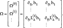
Consider a vehicle, whose configuration is denoted by $ξ_{r} = (x_{r}, z_{r}, θ_{r})$ w.r.t. a fixed reference frame $〈 W 〉,$ that moves on a plane in an unknown environment with the aim of mapping the object point features (or landmarks) and localizing itself with respect to the mapped environmental features. Adopting the notation presented in [6], these landmarks are distinguished between those belonging to objects with unknown position, named targets, and those belonging to objects whose absolute position w.r.t. $〈 W 〉$ is known, which are called markers. We will refer to $ξ_{t} = (ξ_{t, 1}, . . ., ξ_{t, N})$ as a vector with all N targets and $ξ_{m} = (ξ_{m, N + 1}, . . ., ξ_{m, N + M})$ as a vector with all M markers. Wherever necessary, we use the notation $*_{t}$ to specify that the variable refers to a target and $*_{m}$ to specify that it refers to a marker.

The observability problem under analysis is considered in different configurations regarding the number of known and unknown landmarks being observed. The system state variable of the problem at hand comprises the vehicle configuration and the unknown position of the N targets $ξ = (ξ_{r}, ξ_{t}) = (ξ_{r}, ξ_{t, 1}, . . ., ξ_{t, N})$ with dynamic $\dot{ξ} = ({\dot{ξ}}_{r}, 0, . . ., 0)$ (targets are motionless in $〈 W 〉) .$ By noticing that the observable space for a unicycle-like vehicle is a subset of that of an omnidirectional vehicle (the difference is related to the presence of an additional input velocity field), the analysis is carried for the unicycle vehicle. Therefore, assuming that the dynamics are slow enough to be neglected, the vehicle kinematic model is given by ${\dot{ξ}}_{r} = f_{r} (ξ_{r}) = [g_{f} g_{ω}] u_{r},$ where $g_{f} = {[cos θ_{r}, sin θ_{r}, 0]}^{T},$ $g_{ω} = {[0, 0, 1]}^{T}$ and $u_{r} = {[v_{f}, ω]}^{T}$ are the control inputs, i.e., the linear and the angular velocity respectively.

We consider vehicles equipped with a sensor head measuring the angles in the horizontal plane between the line joining the landmark with the head position and the forward direction of the vehicle (see Fig. 1). Of course, a vision system equipped with a simple point feature detection and tracking algorithm falls into this category. The measurement process is modeled by equations of the form

Figure 1.

Fixed frame $< W >,$ vehicle state $(x_{r}, z_{r}, θ_{r}),$ generalized velocities $(v_{f}, v_{h}, ω),$ input disturbances $(d_{f}, d_{h}, d_{ω})$ and $i_{t h}$ landmark position $P_{i} = (x_{i}, z_{i}) .$

y_{i} = h_{i} (ξ_{r}, ξ_{i}) = arctan 2 (\frac{z_{r} - z_{i}}{x_{r} - x_{i}}) - θ_{r} + π,

(1)

where $P_{i} = (x_{i}, z_{i})$ describes the absolute position of the i-th landmark (see Fig. 1). For N targets and M markets, the system output is thus defined as $Y = (y_{t, 1}, y_{t, 2}, . . ., y_{t, N}, y_{m, N + 1}, . . ., y_{m, M + N}) .$ Note that equation (1) is not defined whenever vehicle and landmark positions coincide.

2.2. System Observability

Let us consider a generic continuous time-invariant control affine system $\dot{ξ} = f (ξ) + G (ξ) u$ with system outputs $y = h (ξ),$ where the vector field f is the drift and the matrix G represents the m input velocity fields $G = (g_{1}, . . ., g_{m}) .$ Let the i^th Lie Derivative of a covector field $ω (ξ)$ along a vector field $f (ξ)$ be given by $L_{f}^{(i)} ω$ and let the i^th lie derivative of a generic codistribution $Ω = {[ω_{1} ω_{2} \dots]}^{T}$ along a distribution $Δ = [f_{1} f_{2} \dots]$ be given by $L_{Δ}^{(i)} Ω .$

Let $Δ_{\sum} = (f, g_{1}, . . ., g_{m}),$ and $Ω_{0} = \partial_{ξ} h (ξ)$ be two codistributions. By applying the following iterative formula:

Ω_{k + 1} = Ω_{k} + L_{Δ_{\sum}} Ω_{k},

(2)

the system observability codistribution $d O (ξ) = span [Ω_{\infty}]$ is derived, where $Ω_{\infty}$ is the observability matrix. In [17] it is demonstrated that a nonlinear system is locally weakly observable if the observability rank condition $r a n k (Ω_{\infty}) = \dim (ξ)$ is verified. The analysis here proposed makes use of this notion of observability.

In the rest of the paper we will refer to $Ω^{(i)}$ as the i-th submatrix of Ω that corresponds to the i-th level of Lie Bracketing of (2), i.e., $Ω_{k} = {[Ω^{(0)}, Ω^{(1)}, . . ., Ω^{(k)}]}^{T} .$ Whenever necessary, we will make explicit reference to the terms in $Ω^{(i)},$ i.e., $Ω^{(i)} = [\partial_{ξ 1} L_{Δ_{\sum}} h (ξ), \partial_{ξ 2} L_{Δ_{\sum}} h, . . .],$ for a given $ξ = (ξ_{1}, ξ_{2}, . . .) .$

2.3. Local Decomposition

If a control affine system is not observable in the sense of rank condition [17], there exists a coordinate mapping $ζ = Φ (ξ)$ for which it can be decomposed into observable and unobservable subsystems as follows:

\begin{array}{l} {\dot{ζ}}_{\bar{o}} = f_{\bar{o}} (ζ_{o}, ζ_{\bar{o}}) + g_{\bar{o}} (ζ_{o}, ζ_{\bar{o}}) u \\ {\dot{ζ}}_{o} = f_{o} (ζ_{o}) + g_{o} (ζ_{o}) u, \\ y = h_{o} (ζ_{o}) \end{array}

(3)

where the observable state, i.e., the one that satisfies the rank condition, is given by $ζ_{o}$ and the unobservable state is given by $ζ_{\bar{o}} .$ The local decomposition for linear systems was originally dubbed Kalman observable canonical form.

3. Planar bearing SLAM observability

In this section the planar bearing SLAM observability problem assuming the knowledge of the control inputs is discussed. The results here reported extend those in [6] by detailing all possible cases from 3 + N markers to 3 + N targets, thus including the unobservable cases and the related Kalman Form decomposition.

3.1. Codistribution form

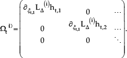
A generic form for the observability codistribution of the systems under investigation is

Ω = [\begin{array}{l} Ω^{(0)} \\ Ω^{(1)} \\ ⋮ \end{array}] = [\begin{array}{l} \partial_{ξ r} h_{1} \partial_{ξ t} h_{1} \\ ⋮ ⋮ \\ \partial_{ξ r} L_{Δ}^{(1)} h_{1} \partial_{ξ t} L_{Δ}^{(1)} h_{1} \\ ⋮ ⋮ \end{array}] .

(4)

In all cases, the rank of the observability codistributions reaches its maximum within the first level of Lie differentiation.

3.2. Observability Analysis

Each feature configuration is now analyzed separately. Before going into details, we recall that the state space of a vehicle moving on a plane has dimension 3, while each landmark has 2 variables w.r.t. the plane of motion.

Case A: 3 or more markers: The observability codistribution rank is equal to 3 for $Ω^{(0)},$ which means that the system is locally weakly observable with level 0 Lie bracketing. Therefore, apart from singular configurations, the problem is statically invertible and reconstruction does not depend on system inputs. Singular configurations are easily determined by analyzing where the codistribution rank is less than 3.

Case B: 2 markers: After 1 level of Lie differentiation, the observability codistribution rank reaches its maximum of 3, apart from configuration singularities, and the system is completely locally weakly observable. The problem is not statically invertible, instead state reconstruction is only possible under vehicle motion.

Case C: 1 and a half markers and half target: For this case, the output function is given by the measurements from two landmarks: one landmark position is completely known (marker); the other landmark position is partially known (half marker), i.e., only one of the 2 plane coordinates is assumed to be known. Without loss of generality, we will assume that the coordinate $z_{i}$ (half marker) is known while $x_{1}$ is unknown (half target). Hence the state space to reconstruct is $ξ = (ξ_{r}, x_{1}),$ while the system output is $y = (y_{1}, y_{m, 2}) .$ After 1 level of Lie differentiation, the observability codistribution rank reaches its maximum of 4, apart from configuration singularities. Hence, all state variables fromξ are locally weakly observable, as the Case B.

Case D: 1 marker: After 1 level of Lie differentiation, the observability codistribution rank reaches its maximum of 2, apart from configuration singularities. Hence, ξ is not fully observable and the unobservable space dimension is 1. From geometric analysis, the unobservable space is given by a circumference centered in the marker.

Kalman form decomposition

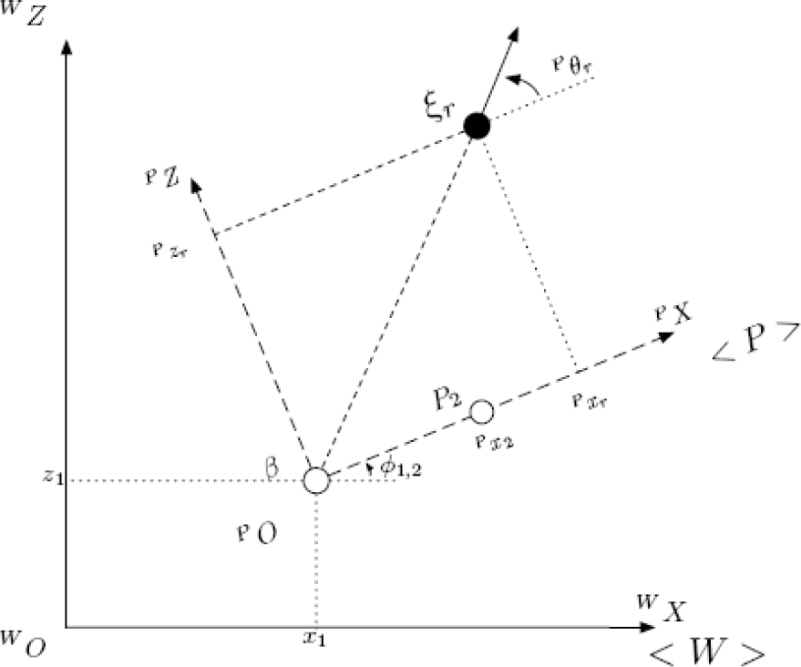
Consider a reference frame $〈 P 〉 = {{}^{P}O, {}^{P}X, {}^{P}Z}$ (see Fig. 2) such that its origin ${}^{P}O$ coincides with the position of the feature $P_{1} = (x_{1}, z_{1})$ and axes ${}^{P}X$ and ${}^{P}Z$ are parallel to axes ${}^{W}X$ and ${}^{W}Z$ respectively. Moreover, consider the coordinates mapping $ζ = Φ (ξ) = {[ρ, β, ϕ]}^{T}$ described by $Φ = ℝ^{2} \times S \to ℝ^{+} \times S^{2},$ which maps the pose displacement between $ξ_{r}$ and $P_{1}$ in polar coordinates w.r.t. $〈 P 〉,$ i.e.,

Figure 2.

Reference frame <P> with axes parallel to <W> and vehicle configuration represented using polar coordinates

ζ = Φ (ξ_{r}) = [\begin{array}{l} ρ \\ β \\ ϕ \end{array}] = [\begin{array}{l} \sqrt{{(x_{r} - x_{1})}^{2} + {(z_{r} - z_{1})}^{2}} \\ {tan}^{- 1} (\frac{z_{r} - z_{1}}{x_{r} - x_{1}}) - θ r + π \\ {tan}^{- 1} (\frac{z_{r} - z_{1}}{x_{r} - x_{1}}) \end{array}],

(5)

where ρ represents the cartesian distance from the vehicle to the point $P_{1}, β$ represents the angle displacement between vehicle orientation and the line that passes through point $P_{1}$ and vehicle position and ϕ represents the angle formed by the vehicle with both axes ${}^{P}X$ and ${}^{W}X .$ Notice that the polar coordinates transformation is undefined for $ρ = 0.$ Vehicle kinematics on polar coordinates is then given by

\dot{ζ} = [\begin{array}{l} - cos (β) \\ \frac{sin (β)}{ρ} \\ \frac{sin (β)}{ρ} \end{array}] v_{f} + [\begin{array}{l} 0 \\ - 1 \\ 1 \end{array}] ω .

(6)

We are now in a position to decouple observable and unobservable subsystems. Indeed, under such coordinate transformation, the system output becomes $y = (β) .$ For $ρ \neq 0$ and after 1 level of Lie differentiation, the observability codistribution for ζ is

Ω = [\begin{matrix} 0 & 1 & 0 \\ - \frac{sin (β)}{ρ^{2}} & - \frac{cos (β)}{ρ} & 0 \end{matrix}],

whose null space is given by

Ker (Ω) = span ({[0, 0, 1]}^{T}) .

Therefore, the observable subsystem is

ζ_{o} = (ρ, β)

and the unobservable subsystem is

ζ_{\bar{o}} = (ϕ) .

In other words, the vehicle is able to determine its distance ρ to the feature and the angle β by which it sees the feature, but its orientation ϕ with respect to a generic reference frame attached to the plane of motion remains unknown.

Case E: Half marker and half target: We are now interested in a robot whose output measurements consist of two landmarks: one landmark has a position that is partially known. Without loss of generality, the coordinate $z_{1}$ (half marker) is assumed known while x₁ is unknown (half target). Again, the state space is $ξ = (ξ_{r}, x_{1})$ and the system output is $y = (y_{1}) .$ After 1 level of Lie differentiation, the observability codistribution rank reaches its maximum of 2, apart from configuration singularities. Hence, ξ is not observable, while the dimensions of the observable and unobservable spaces is 2.

Kalman form decomposition

With reference to the reference frame $〈 P 〉$ presented in section 3.2. 4 and Fig. 2, consider the coordinates transformation $ζ = Φ (ξ) = {[ρ, β, ϕ, x_{1}]}^{T}$ described by $Φ = ℝ^{3} \times S \to ℝ^{+} \times ℝ^{1} \times S^{2},$ i.e., the mapping to polar coordinates (5) plus the half target coordinate. Notice that $x_{1}$ corresponds to the unknown horizontal translation from origin $O_{P}$ to origin $O_{W}$ along ${}^{P}X .$ The system dynamics $\dot{ζ}$ is (6) plus ${\dot{x}}_{1} = 0$ and system output is again $y = (β) .$

Using the new set of coordinates, after 1 level of Lie differentiation, the observability codistribution for ζ is

Ω = [\begin{matrix} 0 & 1 & 0 & 0 \\ - \frac{sin (β)}{ρ^{2}} & \frac{cos (β)}{ρ} & 0 & 0 \end{matrix}],

whose null space is

Ker (Ω) = span ([0_{2 x 2}, I_{2}]),

where we use the notation

0_{i x j}

to represent a

i \times j

matrix of zeros and

I_{i}

an identity matrix of dimension i. As in section 3.2. 4, the observable subsystem is

ζ_{o} = (ρ, β)

and the unobservable subsystem is

ζ_{\bar{o}} = (ϕ, x_{1}),

which means that the horizontal translation

x_{1}

between

O_{W}

and

O_{P}

is unobservable.

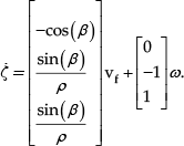
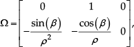
Case F: 1 target: After 1 level of Lie differentiation, the observability codistribution rank reaches its maximum of 2, apart from configuration singularities.ξ is not completely observable and the unobservable space dimension has 3.

Kalman form decomposition

With reference to Fig. 2, consider again the frame $〈 P 〉$ and the mapping $ζ = Φ (ξ) = {[ρ, β, ϕ, x_{1}, z_{1}]}^{T}$ described by $Φ = ℝ^{4} \times S \to ℝ^{+} \times ℝ^{2} \times S^{2} .$ As in section 3.2. 5, $(x_{1}, z_{1})$ corresponds to the position of the origin $O_{P}$ w.r.t $〈 W 〉 .$ The system dynamic has an additional variable ${\dot{z}}_{1} = 0$ and the system output is $y = (β) .$

Using the new set of coordinates, after 1 level of Lie differentiation, the observability codistribution for ζ is

Ω = [\begin{matrix} 0 & 1 & 0 & 0 & 0 \\ - \frac{sin (β)}{ρ^{2}} & \frac{cos (β)}{ρ} & 0 & 0 & 0 \end{matrix}],

whose null space is given by

Ker (Ω) = span ([0_{3 \times 2}, I_{3}])

and we can conclude that the observable subsystem is

ζ_{o} = (ρ, β)

while the unobservable subsystem is

ζ_{\bar{o}} = [ϕ, x_{1}, z_{1}],

i.e., angle ϕ and origin

{}^{P}O

w.r.t. world frame

< W >

are not observable, similar to section 3.2. 4.

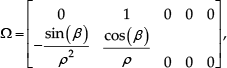
Case G: 2 targets: After 1 level of Lie differentiation, the observability codistribution rank reaches its maximum of 4, apart from singularities. Hence, ξ is not fully observable, with an unobservable subspace dimension of 2.

Kalman form decomposition

Consider a reference frame $< P > = {{}^{P}O, {}^{P}X, {}^{P}Z}$ such that its origin ${}^{P}O$ is coincident to the position of the feature $P_{1} = (x_{1}, z_{1})$ and axis ${}^{P}X$ is coincident to the line that passes through $P_{1}$ and $P_{2}$ , with direction from $P_{1}$ to $P_{2}$ (see Fig. 3 for reference). Orientation of $〈 P 〉$ w.r.t. $〈 W 〉$ will be denoted $ϕ_{1, 2} .$ Position $P_{2}$ w.r.t. $〈 P 〉$ will be described by ${}^{P}P_{2} = {{}^{P}x_{2}, 0}$ and vehicle configuration will be described as ${}^{P}ξ_{r} = ({}^{P}x_{r}, {}^{P}z_{r} {}^{P}θ_{r}) .$

Figure 3.

Reference frame <P> of 2 targets problem

Consider the coordinate transformation $ζ = ({}^{P}x_{r}, {}^{P}z_{r} {}^{P}θ_{r}, {}^{P}x_{2}, x_{1}, z_{1}, ϕ_{1, 2})$ given by $Φ = ℝ^{6} \times S \to ℝ^{5} \times S^{2}$ and defined as

ζ = [\begin{array}{l} (x_{r} - x_{1}) cos ({tan}^{- 1} (\frac{z_{r} - z_{1}}{x_{2} - x_{1}})) + (z_{r} - z_{1}) sin ({tan}^{- 1} (\frac{z_{2} - z_{1}}{x_{2} - x_{1}})) \\ (z_{r} - z_{1}) cos ({tan}^{- 1} (\frac{z_{2} - z_{1}}{x_{2} - x_{1}})) - (x_{r} - x_{1}) sin ({tan}^{- 1} (\frac{z_{2} - z_{1}}{x_{2} - x_{1}})) \\ θ_{r} - {tan}^{- 1} (\frac{z_{2} - z_{1}}{x_{2} - x_{1}}) \\ (x_{2} - x_{1}) cos (ϕ_{1, 2}) + (z_{2} - z_{1}) sin (ϕ_{1, 2}) \\ x_{1} \\ z_{1} \\ {tan}^{- 1} (\frac{z_{2} - z_{1}}{x_{2} - x_{1}}) \end{array}],

for which system dynamic yields

\dot{ζ} = (cos ({}^{P}θ_{r}) v_{f}, sin ({}^{P}θ_{r}) v_{f}, 0, . . ., 0)

and system output becomes

y = [\begin{array}{l} π - {}^{P}θ_{r} + {tan}^{- 1} (\frac{P_{z_{r}}}{P_{x_{r}}}) \\ π - {}^{P}θ_{r} + {tan}^{- 1} (\frac{P_{z_{r}}}{P_{x_{r}} - P_{x_{2}}}) \end{array}] .

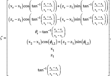
Φ is a not a global diffeomorphism since it is not defined if the robot is on the feature position $P_{1} .$ Moreover, Φ is not defined if ${}^{P}x_{2} = 0,$ i.e., the features are coincident, which is the Case F. After 1 level of Lie differentiation, the observability codistribution for ζ is:

Ω = [\begin{matrix} \partial_{ζ_{r}} h_{1} & 0 & 0 & 0 & 0 \\ \partial_{ζ_{r}} h_{2} & \partial_{ζ_{4}} h_{2} & 0 & 0 & 0 \\ \partial_{ζ_{r}} L_{Δ} h_{1} & 0 & 0 & 0 & 0 \\ \partial_{ζ_{r}} L_{Δ} h_{2} & \partial_{ζ_{4}} L_{Δ} h_{2} & 0 & 0 & 0 \end{matrix}],

where:

\begin{array}{l} \partial_{ζ_{r}} h_{i} = [\frac{^{P} Δ z_{r, i}}{^{P} ρ_{r, i}^{2}} \frac{^{P} Δ x_{r, i}}{^{P} ρ_{r, i}^{2}} - 1], \partial_{ζ_{4}} h_{2} = \frac{^{P} Δ z_{r, 2}}{^{P} ρ_{r, 2}^{2}}, \\ \partial_{ζ_{r}} L_{Δ} h_{i} = {[\begin{array}{l} \frac{2^{P} Δ x_{r, i}^{P} Δ z_{r, i} cos ({}^{P}θ_{r}) + (^{P} Δ z_{r, i} +^{P} Δ x_{r, i}) (^{P} Δ z_{r, i} -^{P} Δ x_{r, i}) sin ({}^{P}θ_{r})}{^{P} ρ_{r, i}^{4}} \\ - \frac{2^{P} Δ x_{r, i}^{P} Δ z_{r, i} sin ({}^{P}θ_{r}) + (^{P} Δ z_{r, i} +^{P} Δ x_{r, i}) (^{P} Δ z_{r, i} -^{P} Δ x_{r, i}) cos ({}^{P}θ_{r})}{^{P} ρ_{r, i}^{4}} \\ \frac{^{P} Δ x_{r, i} cos ({}^{P}θ_{r}) +^{P} Δ z_{r, i} sin ({}^{P}θ_{r})}{^{P} ρ_{r, i}^{2}} \end{array}]}^{T}, \\ \partial_{ζ_{4}} L_{Δ} h_{2} = \frac{(- 2^{P} Δ x_{r, 2}^{P} Δ z_{r, 2} cos (θ_{r}) - (^{P} Δ z_{r, 2} +^{P} Δ x_{r, 2}) (^{P} Δ z_{r, 2} -^{P} Δ x_{r, 2}) sin (θ_{r}))}{^{P} ρ_{r, 2}^{4}} . \end{array}

The null space of Ω is $Ker (Ω) = span ([0_{3 \times 4}, I_{3}]),$ hence the observable subsystem is given by $ζ_{o} = ({}^{P}x_{r}, {}^{P}z_{r} {}^{P}θ_{r}, {}^{P}x_{2})$ and the unobservable subsystem is $ζ_{\bar{o}} = (x_{1}, z_{1}, ϕ_{1, 2}) .$ It is worthwhile to note that the observable subsystem $ζ_{o}$ of the 2 target problem is equivalent to the system investigated in the 1 and a half marker problem if one considers the z position of the half marker zero.

3.3. Extension of results

Results presented in this section are extended to any number of targets. Let $ξ^{*} = (ξ_{r}, ξ_{t, 1}, . . ., ξ_{t, N})$ be a generic system. The system that describes the same problem with additional $\bar{L}$ targets will be written as $ξ = (ξ^{*}, ξ_{t, N + M + 1}, . . ., ξ_{t, N + M + L}) .$ We will use the notation ^* whenever we refer to quantities related to the original system $ξ^{*}$ .

Proposition 1: Consider a system $ξ^{*} = (ξ_{r}, ξ_{t, 1}, . . ., ξ_{t, N}),$ for which the dimension of the observable space is given by dim $(ζ_{o}^{*}) = K .$ Now, consider a system $ξ = (ξ^{*}, ξ_{t, N + M + 1}, . . ., ξ_{t, N + M + L})$ that comprises $ξ^{*}$ and L new targets. The dimension of the observable space of ξ is dim $(ζ_{o}) \geq K + L .$

Proof: Given a generic observability codistribution $Ω^{*}$ associated to $ξ^{*} :$

Ω^{*} = (\begin{array}{l} Ω^{*}^{(0)} \\ Ω^{*}^{(1)} \\ ⋮ \end{array}),

the correspondent Ω (associated to ξ) that consider the same problem with

\bar{N}

new targets can be written as

Ω = (\begin{matrix} Ω^{*}^{(0)} & 0 \\ * & Ω_{t}^{(0)} \\ Ω^{*}^{(1)} & 0 \\ * & Ω_{t}^{(1)} \\ ⋮ & ⋮ \end{matrix}),

where

Ω_{t}^{(i)} = (\begin{matrix} \partial_{ξ_{t, 1}} L_{Δ}^{(i)} h_{t, 1} & 0 & \dots \\ 0 & \partial_{ξ_{t, 1}} L_{Δ}^{(i)} h_{t, 2} & \dots \\ 0 & 0 & ⋱ \end{matrix}) .

Given that

{Ω_{t}^{(0)}, Ω_{t}^{(1)}}

has rank 2, we can conclude that

rank (Ω) \geq rank (Ω^{*}) + L .

Table 1.

Observability analysis summary: M – Number of markers; N – N Number of targets; K – Minimum level of lie-bracketing required to cover observable space; n – System dimension; $n_{o}$ – Observable space dimension; $n_{\bar{o}}$ – Unobservable space dimension

M	0	0 0 0	1	1+1/2	1+1/2	2	3+M̄
N	2+N̄	2 1	1/2	0 0	N̄	0	N̄
k	1	1 1 1	1 1	0	1	0
n	7+2N̄	7 5 4	3 4	4+N̄	3	3+2M̄+2N̄
n_o	4+2N̄	4 2 2	2 4	4+N̄	3	3+2M̄+2N̄
n_ō	3	3 3 2	1 0	0	0 0

Corollary 1: If $ξ^{*}$ is completely observable then ξ is completely observable.

Table I presents an overview of the results obtained in this section for any number of targets.

4. Results

Theoretical results were evaluated by simulations, implementing the nonlinear observer described in [16] to reconstruct the observable space of the cases analyzed in section 3. Simulation results for arbitrary configurations are summarized in Fig. 4. Notice that the nonlinear observer converges in all cases, hence it always succeeds in reconstructing the observable space.

Figure 4.

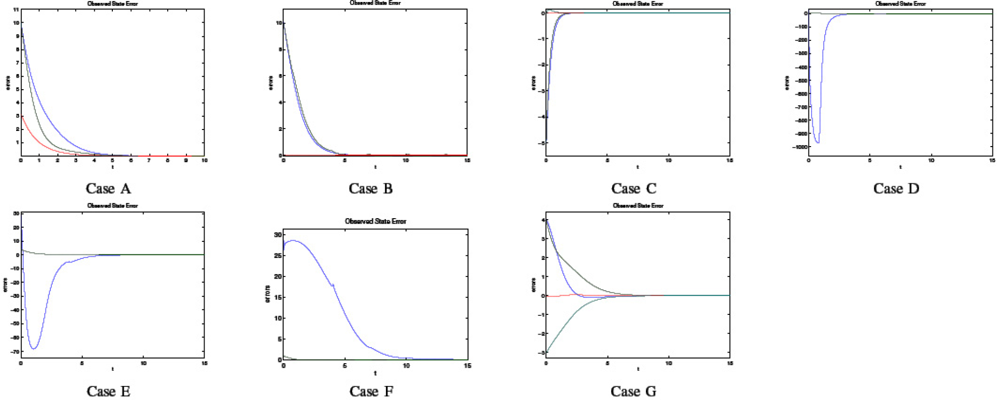
Observed state errors $e_{o} = ζ_{o} - {\hat{ζ}}_{o}$

In particular, when only one landmark is being observed (Case D,E and F), the observable subsystem is $ζ_{o} = (ρ, β)$ where ρ represents the cartesian distance of the vehicle from the landmark and β represents the bearing angle between the vehicle orientation and the landmark. The unobservable space in these cases is the angle ϕ formed by the vehicle position and any arbitrary reference frame and the position of the landmark if it is a target.

When 2 landmarks $P_{1}$ and $P_{2}$ available (Case B, C, G), the observable subsystem is $ζ_{o} = ({}^{P}x_{r}, {}^{P}z_{r}, {}^{P}θ_{r}, {}^{P}x_{1}, {}^{P}z_{1}, {}^{P}x_{2}, {}^{P}z_{2}, {}^{P}x_{3}, {}^{P}z_{3}, . . .)$ where $〈 P 〉$ is a right-handed coordinate frame whose origin is coincident with the position $P_{1}$ and axis ${}^{P}X$ parallel to the line that passes through $P_{1}$ and $P_{2} .$ If 3 or more landmarks are known (Case A), static complete observability is available, otherwise full observability is reached after 1 level of Lie differentiation. The unobservable space concerns the coordinate transformation between frame $〈 P 〉$ and world frame $〈 W 〉 .$ This coordinate transformation is completely unobservable if all landmarks are targets (Case G), while it is completely observable when at lest three coordinates of the landmark positions are known (Case C), e.g., position of $P_{1}$ and orientation of the line passing through $P_{1}$ and $P_{2}$ w.r.t. $〈 W 〉 .$

4.1. Visual Servoing

In this section we validate the use of the nonlinear observer described in [16] in a Position Based Visual Servoing scheme (as seen in Fig. 5) for the case of measuring 3 markers (as seen in section 3.2. 1). The controller used is the Visual-Servoing with Omnidirectional Sight as presented in [18].

Figure 5.

PBVS Visual Servoing Scheme

The desired configuration of the robot is considered to be coincident to the origin of the world framehWi. The initial vehicle configuration is $ξ_{r} = {100 c m, 100 c m, 0^{\circ}} .$ Landmark positions, control and observer constants are arbitrarily chosen. Measurement noise is not considered.

Results can be seen in Fig. 6. The simulation clearly shows that the pose regulation is successfully achieved.

Figure 6.

Visual Servoing Results: Observer error $e_{o}$ (a); Position error: distance from desired position (b); Orientation error (c); and vehicle trajectory

5. Conclusions and future work

In this paper we have presented a complete observability analysis of the planar bearing only localization and mapping problem for all configurations of landmarks with known (markers) and unknown position (targets). Theoretical results are supported by simulations.

Future work will concentrate mainly on the singularity analysis and on observability without input knowledge.

Footnotes

6. Acknowledgements

The research leading to these results has received funding from the European Union Seventh Framework Programme [FP7/2007-2013] under grant agreement n257462 HYCON2 Network of excellence.

References

Lowe

, and Little

, “Mobile robot localization and mapping with uncertainty using scale-invariant visual landmarks,” International Journal of Robotics Research, vol. 21, pp. 735–758, 2002.

Hartley

and Zisserman

, Multiple View Geometry in Computer Vision. Cambridge University Press, 2003.

Corke

, Mobile Robot Navigation As A Planar Visual Servoing Problem. Springer Berlin Heidelberg, 2003, vol. 6, pp. 361–372.

Danesi

Fontanelli

, and Bicchi

, “Visual servoing on image maps,” in Experimental Robotics, ser. Springer Tracts in Advanced Robotics, Khatib

Kumar

, and Rus

, Eds. Springer Berlin / Heidelberg, 2008, vol. 39, pp. 277–286.

Silveira

Malis

, and Rives

, “An efficient direct approach to visual slam,” Robotics, IEEE Transactions on, vol. 24, no. 5, pp. 969–979, 2008.

Bicchi

Prattichizzo

Marigo

, and Balestrino

, “On the observability of mobile vehicle localization,” in Proc. IEEE Mediterranean Conf. On Control And Systems, 1998.

Bicchi

Lorussi

Murrieri

, and Scordio

, “On the problem of simultaneous localization, map building, and servoing of autonomous vehicles,” in Advances in Control of Articulated and Mobile Robots, ser. Springer Tracts in Advanced Robotics Siciliano

Melchiorri

De Luca

, and Casalino

, Eds. Springer Berlin / Heidelberg, 2004, vol. 10, pp. 144–144.

Xin

Xiao

, and You

;, “Research on unobservability problem for two-dimensional bearings-only target motion analysis,” in Proc. of 2005 International Conference on Intelligent Sensing and Information Processing, Jan 2005, pp. 56–60.

Martinelli

Pont

, and Siegwart

, “Multi-robot localization using relative observations,” in Proc. IEEE International Conference on Robotics and Automation (ICRA'05), april 2005, pp. 2797–2802.

10.

Martinelli

and Siegwart

, “Observability properties and optimal trajectories for on-line odometry self-calibration,” in 2006 45th IEEE Conference on Decision and Control, Dec 2006, pp. 3065–3070.

11.

Sert

Kökösy

A. M.

and Perruquetti

, “A single landmark based localization algorithm for non-holonomic mobile robots,” in ICRA, 2011, pp. 293–298.

12.

Soatto

, “3-d structure from visual motion: Modeling, representation and observability,” Automatica, vol. 33, pp. 1287–1312, 1997.

13.

Nister

Naroditsky

, and Bergen

, “Visual odometry,” in Proc. of the 2004 IEEE Computer Society Conference on Computer Vision and Pattern Recognition (CVPR'04), vol. 1, Jan 2004, pp. I–652–I–659 Vol.1.

14.

Nister

O. N. D.

and Bergen

, “Visual odometry for ground vehicle applications,” Journal of Field Robotics, vol. 23, 2006.

15.

Davison

, “Real-time simultaneous localisation and mapping with a single camera,” in Proc. of the Ninth IEEE International Conference on Computer Vision – Volume 2, Jan 2003.

16.

Belo

F. A. W.

Salaris

, and Bicchi

, “3 known landmarks are enough for solving planar bearing slam and fully reconstruct unknown inputs,” in Proc. IEEE International Conference on Intelligent Robots and Systems (IROS'10), 2010.

17.

Hermann

and Krener

, “Nonlinear controllability and observability,” IEEE Trans. on Automatic Control, vol. 22, no. 5, pp. 728–740, Jan 1977.

18.

Fontanelli

Salaris

Belo

F. A. W.

, and Bicchi

, “Unicycle– like robots with eye-in-hand monocular cameras: From pbvs towards ibvs,” in Visual Servoing via Advanced Numerical Methods. Springer Berlin / Heidelbergp, 2009.

A Complete Observability Analysis of the Planar Bearing Localization and Mapping for Visual Servoing with Known Camera Velocities

Abstract

Keywords

1. Introduction

2. Problem definition

2.1. System Dynamics

2.2. System Observability

2.3. Local Decomposition

3. Planar bearing SLAM observability

3.1. Codistribution form

3.2. Observability Analysis

3.3. Extension of results

4. Results

4.1. Visual Servoing

5. Conclusions and future work

Footnotes

6. Acknowledgements

References