
Abstract
To solve the view visibility problem and keep the observed object in the field of view (FOV) during the visual servoing, a depth adaptive zooming visual servoing strategy for a manipulator robot with a zooming camera is proposed. Firstly, a zoom control mechanism is introduced into the robot visual servoing system. It can dynamically adjust the camera's field of view to keep all the feature points on the object in the field of view of the camera and get high object local resolution at the end of visual servoing. Secondly, an invariant visual servoing method is employed to control the robot to the desired position under the changing intrinsic parameters of the camera. Finally, a nonlinear depth adaptive estimation scheme in the invariant space using Lyapunov stability theory is proposed to estimate adaptively the depth of the image features on the object. Three kinds of robot 4DOF visual positioning simulation experiments are conducted. The simulation experiment results show that the proposed approach has higher positioning precision.
1. Introduction
The introduction of visual servoing techniques would increase the diversity and extend the application fields of a robot. The aim of robot visual servoing is to control the relative pose of the robot's end-effector, with respect to the manipulated object, using real-time visual information captured from a camera, which is either fixed in the robot work space (eye-on-hand configuration) or mounted at the robot's end-effector (eye-in-hand configuration). In the last few years, many robot visual servoing methods have been proposed to solve the problem of robot positioning and tracking with respect to the manipulated object in the dynamic and unknown environment. These methods can be roughly classified into three types according to the definition of the system error function: position-based visual servoing (PBVS), image-based visual servoing (IBVS), hybrid visual servoing (HVS or 2.5D VS). Each kind of visual servoing method has its own pros and cons. A comprehensive review paper about robot visual servoing can be found in [1].
The basic requirement of these visual servoing algorithms is to keep the observed object in the field of view of the camera during the visual servoing (also known as the visibility problem). When the robot initial position is far from the desired position, the object could leave the camera field of view during the visual servoing. This will cause the visual servoing task to fail and limit its further application [2, 3]. There are two kinds of common solutions to this view visibility problem: trajectory planning and active vision techniques such as active zoom control. The main idea of trajectory planning is to plan the trajectories of a set of features points on the object in the image space and then to track these trajectories. At present, many trajectory planning methods have been proposed. In general these methods would be roughly classified into four types: image space-based planning [5], global path planning [6], optimization-based planning [7] and potential field-based planning [8]. Tracking a planned trajectory can keep the change of the robot pose in a small range. Thus, it would be possible to keep the object in the camera field of view by enforcing such constraints on the trajectories [4] and the visibility problem could be solved. However, this kind of method is sensitive to the change of the camera intrinsic parameters. A comprehensive review paper about trajectory planning can be found in [9].
Another solution is to combine the active vision technique with the robot visual servoing system, e.g., an active zoom control technique. The main idea of active zooming could be described as follows:
Zooming out when one of the interest points, which are also called the features points on the object, is close to leaving the image.
Zooming in when the interest points are well centred in the image, to get good resolution of the interesting points.
It can be seen that active zoom control could not only solve the view visibility problem, but also improve the accuracy of the features extraction from the interest object and the precision of the whole robot visual servoing system [2]. This has been widely used in the computer vision field [10, 11]. For example, Kumar et al. constructed a stereo vision system through the two pant-tilt-zoom (PTZ) cameras and localized a moving target precisely in a complex and large environment [11]. If we combine the active zooming idea with the robot visual servoing method, we could solve the view visibility problem in robot visual servoing and improve the accuracy of the whole visual servoing system. However, it is difficult to apply this active vision technique directly to traditional visual servoing approaches because traditional visual servoing approaches are based on a teaching-by-showing technique. This means that we must first store the desired image captured in the desired position and then control the robot, starting at another position than the desired position, where the current image coincides with the desired image. In other words, traditional visual servoing methods are “camera-dependent”. To solve this “camera-dependency” problem, one good solution is to employ the invariant visual servoing (or intrinsic-free visual servoing) method proposed in [12]. The key idea of invariant visual servoing is to construct a system error function using a projective invariant property. The error function is invariant to the changes in camera intrinsic parameters and only relevant to the relative position and pose between camera and object. An image Jacobian matrix in the error function describes the relationship between the camera velocity and the image features error in the invariant space. This invariant visual servoing approach provides a good methodology for controlling the robot with a zooming camera, but it cannot be used on a planar object. In addition, it doesn't consider the focus length control problem. This means that we can control the robot using a different focus length to the one used in the learned stage, but we can't control or change the focus length during the visual servoing. In order to deal with this problem, a zooming visual servoing method is proposed in [13]. This method allows us to control the focus length during the visual servoing by using a focus length control strategy and then recover the focus length value corresponding to the desired image at the end of the visual servoing. In addition, this method can also solve the planarity problem from the method proposed in [12]. However, the methods proposed in [12 and 13] do not take into account depth estimation problems and estimate the object depth at the very beginning of the visual servoing, then keep it constant throughout. However, the image Jacobian matrix depends on the depth parameter, which is a time-varying parameter, so a constant depth estimation value could only locally guarantee the convergence of the method. In order to further improve the invariant visual servoing method proposed in [12 and 13], we proposed a nonlinear depth adaptive estimation algorithm using Lyapunov stability theory in the invariant space. Some depth estimation algorithms using Lyapunov stability theory have been proposed in the past years [14, 15]. These estimation methods can work well in the case of the fixed camera intrinsic parameters but can not be used in the case of the variant camera intrinsic parameters. In this paper we extend these depth estimation methods to zooming visual servoing, where the camera intrinsic parameter changes during the visual servoing and gives a detailed derivation. Finally, we design a zooming visual servoing strategy for a manipulator robot with a zooming camera. Simulation results show that our approach has a better convergence performance of the image error.
The remaining part of this paper is organized as follows. The basic principle of the invariant visual servoing method is briefly introduced in Section 2. The details of our algorithm are described in Section 3, where we propose an efficient depth adaptive zooming visual servoing approach. Simulation results and analysis are given in Section 4. Section 5 will conclude the paper by discussing the proposed approach and suggest some improvements for further research.
2. Basic Principles of Invariant Visual Servoing
In this section, we briefly introduce the basic principles of the invariant visual servoing method, related space notations and a pin-hole imaging model.
2.1 Space Notations
The 3D points, with homogeneous coordinates χi = (Xi,Yi,Zi,1) (i = {1,2,…n}) are projected in the absolute camera frame F* to the points

where Zi is the positive depth and
2.2 Camera Model
The image point

where
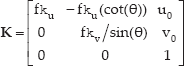
f is the focal length (in metres), ku and kv separately are the magnifications in the ↑ and ↕ direction (in pixels/m), u0 and v0 are the coordinates of the principle point (in pixels) and θ is the angle between ↑ and ↕ axes.
2.3 Basic Principle of the Invariant Visual Servoing
The main idea of the invariant visual servoing proposed in [12] is to construct an error function, which is independent of the changes in camera intrinsic parameters and θ is only dependent on the relative pose of the camera/robot, with respect to an observed object on the invariant space. The image Jacobian matrix in the error function describes the relationship between the camera velocity and image features error in the invariant space. Then the visual servoing law can be designed by the error function. Therefore, the construction of the invariant space and image Jacobian matrix are two important elements for invariant visual servoing.
2.3.1 Construction of the Invariant Space
The aim of the construction of the invariant space is to keep the features points invariant to the camera intrinsic parameters. The whole construction process can be divided into five steps as follows.

Non-singular matrices
Image feature point p and p* in the original image space can be converted into the invariant image feature point and


From the equations above we know that both
2.3.2 Construction of the Image Jacobian Matrix in the Invariant Space
Just like in the IBVS (image-based visual servoing) approach, the camera is now controlled in the invariant space. The derivative of the vector


By plugging Equation (6) into the above equation, we can get:
Since

According to the IBVS we know the derivative of the current image point is

where
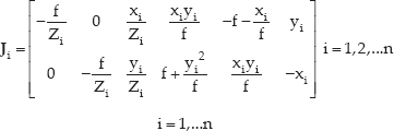
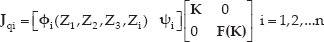
Where,


2.3.3 Definition of the error function in the Invariant Space
The error function in the invariant space can be defined as follows:

whare

where λ is a positive scalar factor, the robot can be driven back to the desired position only if
3. Basic principle of the depth adaptive zooming visual servoing
The invariant visual servoing approach described above provides a good methodology to control the robot with a zooming camera. In this section, we will bring the zoom control and depth adaptive estimation into the invariant visual servoing method and proposed a depth adaptive zooming visual servoing method. The purpose of the proposed method is to keep the observed object always staying in the field of view of camera during the visual servoing through change the camera focus length, and to adaptively estimate the depth of the image feature points on the object during the visual servoing.
3.1 The Basic Structure of the Depth Adaptive Zooming Visual Servoing
The whole servoing structure diagram of the proposed robot depth adaptive zooming visual servoing method can be depicted in Fig. 1. The desired input
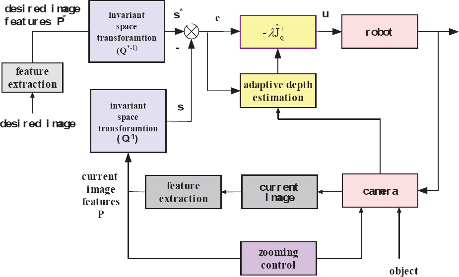
Structure diagram of depth adaptive zooming visual servoing.
3.2 Zooming Control
The purpose of zooming control can be described as follows:
During the robot visual positioning process, zooming out when the object moves away from the camera (even out of the field of view) and zooming in to produce an expanding image of the interest object can achieve high precision positioning [17–19]. Note that the zooming control can't change the resolution of the image captured from the camera, but can change the local resolution of the interest object.
First, we define δ as the distance from the nearest feature point on the object to the border of the image plane. δ = min(ui, vi, umax -ui, vmax -vi), where umax and vmax are respectively the image dimensions in the ↑ and ↕ direction. We can control the zoom in order to keep the nearest point to the image borders at a given distance. The zooming areas in the image plane are shown in Fig. 2.
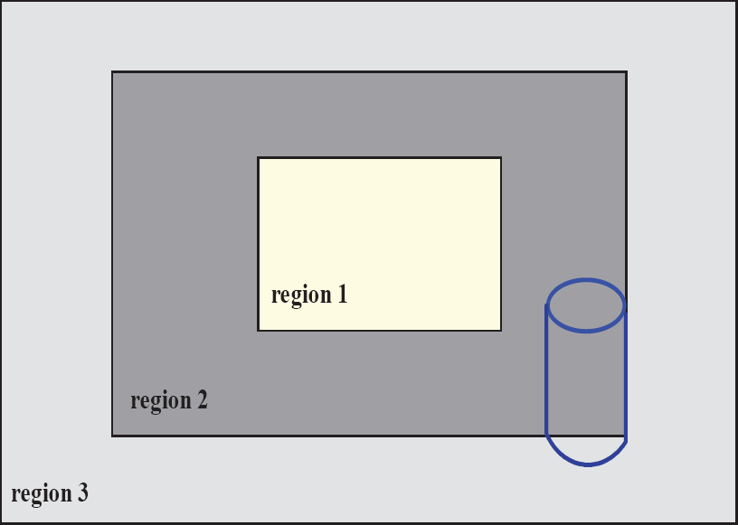
Zooming areas.
If the object is in region 1, i.e., δ is in section 1, in order to improve the image resolution of the interest object, we can enlarge the focal length. Zooming means

If the object is in the dark grey area, i.e., δ is in region 2, there is no zooming in this area which can keep all the feature points in the view of the camera stably. That is
If the object is in the light grey area, i.e., δ is in region 3, it means that the object will escape from the field of view of the camera, so we should decrease zoom in this area to obtain a sufficient field of view of the camera. The corresponding mathematical expression can be written as

According to the different regions where the object is, we can adopt the corresponding zooming control rules to improve the image resolution on the premise of guaranteeing all the features on the object stay in the field of view of the camera.
3.3 Depth Adaptive Estimation
As the description in subsection 2.3 states, the visual servoing law is
We define the function of the whole state (

where
In order to ensure system stability, we must address the system satisfy Lyapounov theories.
Observing the matrix
By expanding Equation (15), we can observe:
The derivative of Equation (16) is:

If we use the depth adjusting law:

Where, γ1 > 0, γ2 >0,i = 1,2,…,n,
So Equation (17) can be simplified as follows:
where:

The camera velocity
If we define the vector

where
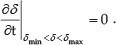
We know that V ≥ 0. If V̇ ≤ 0 in a region then the system with the adaptive estimation method is locally asymptotically stable. If:

where

meaning that the state error
As the unknown object depth, if the visual servoing law is
4. Simulation Results
In this section we build a robot depth adaptive zooming visual servoing simulation model in a MATLAB environment, based on Peter's robotics toolbox [20] and conduct three kinds of robot visual positioning simulation experiments to validate the performance of the proposed depth adaptive zooming visual servoing.
The first simulation experiment aims to demonstrate the rationality of the whole structure with zooming control. The second simulation involves plugging into the depth adaptive method and is in contrast with the first simulation, in order to validate the visual servoing performance of the proposed approach. The third simulation aims to demonstrate the validity of the proposed approach in a different initial position.
4.1 Related Parameter Settings
The camera is in the eye-in-hand configuration. The related parameters used in the simulation experiments are as follows:
the number of the feature points n=12
coordinates of the principle point u0=256, v0=256 (in pixels)
magnifications in the direction ↑ and ↑ ku =20000, k v =20000 (in pixels/m)
angle between u and v axes” 0=90°
initial focal length f0=0.015 (in meters)
desired focal length fd=0.012 (in meters)
coordinates of the 12 image points in the 3D space with different depth points=
[0.5–0.5 2.01; 0.9 0.2 2.04;-0.2–0.2 2;
0.9–0.5 2.01; 0.9–0.9 2.01; 0.5–0.9 2.01;
0.7–0.7 2.01; 0.5–0.2 2.04; 0.7 0 2.04;
0.2 0.2 2; 0.2–0.2 2; −0.2 0.2 2],
the initial camera pose

Suppose the robot move 700mm in the X-minus direction, 300mm in the Y direction, 100mm in the Z-minus direction and take the rotation −0.3rad along the Z direction. Then we get the goal position:

The visual servoing law used is
We don't consider the depth estimation in the first simulation experiment, but consider the depth estimation, with the depth adjusting gains γ1 = 102, γ2 =103 in the second simulation.
4.2 Results and Discussion
4.2.1 Simulation experiment 1: robot zooming visual servoing without depth estimation
In this simulation experiment, 12 image feature points on the target object at the desired position and at the initial position are obtained respectively. Then the robot moves from the initial position to the desired position using zooming visual servoing without depth estimation. The motion trajectory of the 12 feature points in the image plane is shown in Fig. 3. At the very beginning of the servoing, the focal length is 12mm and there are four points outside of the field of view. The camera zooms out in order to assure the interest object points are all in view at the beginning of the servoing. During the late servoing, zooming in improves the image resolution and the final focus value is 17.3mm (Fig. 5 (b)). The simulation results show that the control method can make the error of characteristic vectors in invariant space of the target object zero (Fig. 5 (a)). As a consequence, the positioning error in directions X, Y and Z are Xerror=1.66mm, Yerror=0.59mm, Zerror=6.44mm, respectively. The rotation error converges to 0 (Fig. 4 (a) and Fig. 4 (b)). So the robot can reach the desired position.
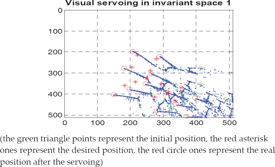
The image points trajectory (blue points) without depth estimation.

Visual positioning error without depth estimation; (a) Translation error. (b) Rotation error around Z axes.

Error in the invariant space and change of focal length without depth estimation; (a) The total error in the invariant space. (b) Focal length changes in visual servoing.
4.2.2 Simulation experiment 2: robot zooming visual servoing with depth adaptive estimation
In this section, we conducted another robot 4DOF visual positioning simulation experiment using zooming visual servoing with a depth adaptive estimation method. The experiment parameters used in this experiment are the same as the ones used in the first simulation experiment. The visual positioning results using zooming visual servoing with a depth adaptive estimation are shown in Fig. 6 – Fig. 8. The motion trajectory of the 12 feature points in the image plane is shown in Fig. 6.
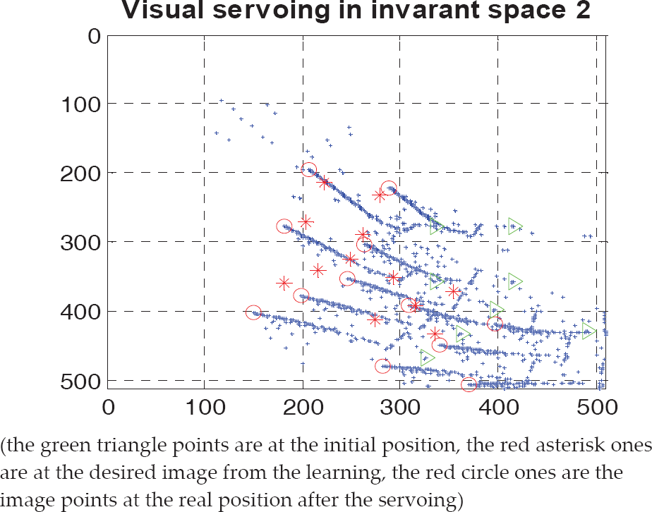
The image points trajectory (blue points) with depth estimation

Visual positioning error with depth estimation

Error in the invariant space and change of focal length with depth estimation; (a) The total error in the invariant space; (b) Focal length changes in visual servoing.
The errors of the characteristic vectors in the invariant space of the target object are zero (Fig. 8 (a)) and the focal lengths finally converge to 17.1mm (Fig.8 (b)). The errors along the X, Y and Z axes are Xerror=0.29mm, Yerror=0.35mm and Zerror=2.59mm. The rotation errors converge to 0 and are shown in Fig.7 (a) and Fig.7 (b) respectively. The simulation results show that the positioning error along the Z axis is smaller when depth estimation is considered in the zooming visual servoing. The whole depth converge process is shown in Fig. 10. Comparison results of the convergence performance of the two zooming visual servoing methods are shown in Fig. 9. It can be seen from the Fig. 9 that the zooming visual servoing with a depth adaptive estimation method has a better convergence performance.

Comparison of the convergence of the two zooming visual servoing method
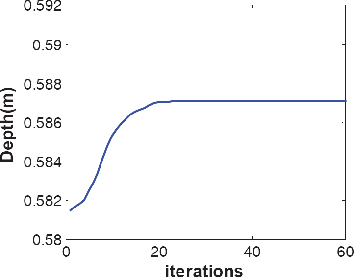
Depth convergence curve
4.2.3 Simulation experiment 3: robot zooming visual servoing with depth adaptive estimation in the different initial position.
In order to demonstrate the validity of the proposed approach further. We conduct another robot 4DOF visual positioning simulation experiment with a different initial camera pose.
Suppose the robots moves 300mm in the X-minus direction, 200mm in the Y direction and −200mm in the Z-minus direction.
Then we get the new initial camera pose:

Other experimental parameters used in this experiment are the same as the ones used in the first two simulation experiments.
The visual positioning results using zooming visual servoing with depth adaptive estimation in the different initial camera position are shown in Fig. 11 – Fig. 13.

Visual positioning error in the different initial camera position

Error in the invariant space and change of focal length in the different initial camera position; (a) The total error in the invariant space; (b)Focal length changes in visual servoing.

Depth convergence curve in the different initial camera position
The translation errors along the X, Y and Z axes and the rotation error around the Z axis are shown in Fig. 11 (a) and Fig. 11 (b) respectively. The errors of characteristic vectors in the invariant space of the target object are zero (Fig. 12 (a)) and the focal length finally converge to 17.1mm in Tcamera_0 and 23.0mm in Tcamera_1 (Fig. 12 (b)). The whole depth convergence process is shown in Fig. 13. The simulation results show that our approach has good visual positioning performance in the different camera initial positions.
The simulation results show that the zoom control method can be used in the invariant visual servoing system. The purpose of the zooming control is to extend the camera's field of view when the target is moving out of range and improve the local resolution of the object of interest when the target is in range of the camera view. In addition, the proposed depth adaptive zooming visual servoing method can guarantee closed-loop stabilization to achieve the 4-DOF robot visual positioning task. It can be seen from Table 1, in contrast to simulation 1, the second simulation system with a depth adaptive estimation has higher visual servoing precision and the whole state of the robot visual servoing system is bounded, though the depth converges to a stable value instead of the true value.
The translation convergence errors along X, Y, Z axes in the two simulations experiments.

The translation convergence errors along X, Y, Z axes in the two different camera initial positions.

5. Conclusion
In this paper, a depth adaptive zooming visual servoing method is proposed to solve view visibility problems. In order to enlarge the field of view, the visual servoing system in the invariant space with zooming control is performed. This could improve the accuracy of image resolution of the target. In order to overcome the defects of the constant depth method, a nonlinear depth adaptive estimation method for robot zooming visual servoing is proposed. With robustness in the invariant space, this adaptive method can improve the accuracy of the servoing system under the zooming condition. The adaptive adjustment mechanism can guarantee that the states of its system are uniformly bounded. The simulation results of robot 4DOF visual positioning show that the proposed method has a better convergence performance for the image error.
No specific feature extraction algorithm is considered in the simulation experiment and some simulation points are defined as the image feature points. The performance of the feature point's extraction will affect the final robot visual servoing. In some cases, the whole robot visual servoing would become unstable, if there is a big mistake while extracting these points. Changing lighting conditions would affect the performance of the feature point's extraction. In addition to a robot/camera system with eye-in-hand configuration, the image captured by the camera will undergo some deformations because of the change in robot pose and camera focus length during the robot zooming visual servoing. These deformations can be locally well approximated by affine transformations of the image plane. In the future, we will apply the affine invariant feature extraction algorithm [21, 22] to extract the affine invariant feature points on the object and extend the proposed robot depth adaptive zooming visual servoing method to real nature scenes.
Footnotes
6. Acknowledgment
This work is supported by the National Natural Science Foundation of China under Grant No. No. 61203345, No. 61174101, the Shaanxi Provincial Natural Science Foundation of China under Grant No. 2009JQ8011 and Educational Commission of Shaanxi Province of China under Grant No. 2010JK737.