Sage Journals: Discover world-class research

Abstract

This paper mainly solves the problem of 2D minimally persistent formation control in which three co-leaders are in a cycle, which raises a great challenge in the area of persistent formation control. First, a novel control law is proposed for this problem. The fundamental moving principles of the agents are well-designed based on the property of persistence, and the non-square rigidity matrix is converted into the square one for the design of the control law. Then, the method of leading principal minor is utilized to prove that the formation with the above control law can be stabilized. Finally, simulation results show that the proposed controllers are able to stabilize the group formation to a rigid shape, while keeping the distances between the agents to the desired value.

Keywords

Three-co-leader Minimally Persistent Formation Rigidity Matrix

1. Introduction

In recent years, many research papers [1 –10] have indicated different ways of solving the problem of fulfilling tasks using a formation. This paper however proposes a minimally persistent formation controller to maintain the distance of the agents continuously based on the concept of rigid control [11, 12]. Furthermore, different from the previous work, what we are dealing with is formation control based on a directed graph, rather than undirected. This type of the rigid formation has been termed as the persistent formation [13 –23].

The underlying graph of the directed formations may be either cyclic or acyclic. Formation control with an acyclic graph is easy dealt with because of its particular structure, where the follower agents cannot influence the leader agents. However, formation control with a cyclic graph has well-known difficulties, since the control of the leader agents may be affected by the follower [18]. In the area of distance maintenance control with a cyclic graph, some authors have made some contributions [15, 23 –25]. Baillieul [19] proposed a method of formation control considering the distance measurements in a cyclic structure, but he did not research how to maintain the distance of all the agents. Hendrix [15] then discussed the possibility of keeping the distance between every pair of agents constant in a cycle graph and raised the concept of minimally persistent formation, but the specific control of the whole formation was not analysed. Furthermore, Yu [17] researched the special control law in a minimally persistent formation with a leader-first-follower variety in the plane and tried to design the control law using a rigidity matrix. However, he only considered the one-leader situation in which the followers are in a cycle. Moreover, in the research of leaders in a cycle, Anderson [25] considered a control law for a formation with only three agents named three co-leaders, but he did not explain the topology relationship of the followers.

To the best of our knowledge, all the aforementioned papers share the following common drawbacks: one-leader model for minimally persistent formation cannot complete the complex mission very soon and it is difficult for one leader to find out the goal in a complicated environment as soon as possible. Consequently, the one-leader model is an important factor limiting the performance of the whole formation. In addition, all the algorithms based on the one-leader model seem to have poor scalability and lack adaptability and flexibility to both tasks and environment.

To overcome the aforementioned drawbacks, a multi-leader architecture is necessary. Yu [17] mentioned that only the minimally persistent formation systems with three leaders can be stabilized. Therefore, the problem of minimally persistent formation control with three co-leaders is discussed in this paper. In the three co-leader model, the three co-leaders are equivalent. In addition, the non-square rigidity matrix, which indicates the distance of all the agents, is introduced in the design of the control law to deal with the timeliness problem.

The primary contribution of this paper is the proposing of a novel control law using a non-square rigidity matrix for minimally persistent formations, in particular, under the condition that the three co-leaders are in the cycle. Firstly, since the leaders and followers have different types of the moving principle, we devise different control laws for them respectively. Secondly, during the course of designing the control laws, the novel method of converting the non-square rigidity matrix into the square one is discussed in detail. Thirdly, it is necessary to consider the situation where the followers are in a cycle and when they are not. Finally, we do the simulations in which the followers are in the acyclic and cyclic graphs to prove the efficiency of the proposed control law.

2. Preliminaries

2.1 Graph rigidity

Before introducing persistent formations in a directed graph, it is necessary to know the underlying rigid formations in an undirected graph. Let G = (V,E) be an undirected graph with n vertices; denote the composite vector p=(p₁,p₂,…p_n)∈R²ⁿ and a pair (G,p). p_i(i∈{1,2,…,n}) represents the coordination of the ith vertex in the place.

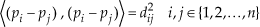
Denote the constant parameter d_ij=|p_i-p_j| as the Euclidean distances between pairs of points (p_i,p_j). In addition, the introduction of the rigidity matrix in [11] claims that:

⟨ (p_{i} - p_{j}), (p_{i} - p_{j}) ⟩ = d_{i j}^{2} i, j \in {1, 2, \dots, n}

(1)

Assume that the trajectory is smooth, then we could get the following expressions from (1):

\begin{array}{l} 2 〈 (p_{i} - p_{j}), (\overset{\cdot}{p_{i}} - \overset{\cdot}{p_{j}}) 〉 = 0, \\ i, j \in {1, 2, \dots, n}, t \geq 0 \end{array}

(2)

where p_i is the velocity at point p_i. Then, we obtain the following homogeneous equation by combining (2) at different points:

R \overset{\cdot}{p} = 0

(3)

where ṗ=column{ṗ₁,ṗ₂,…ṗ_n} and R is called the rigidity matrix with dimension mx2n [m = n(n-1)/2] in the plane.

In addition, the rigidity function is described as follows for another definition of rigidity matrix:

{\overset{\land}{g}}_{G} (p) = {[| | p_{e_{1}}^{i n} - p_{e_{1}}^{o u t} | |^{2}, | | p_{e_{2}}^{i n} - p_{e_{2}}^{o u t} | |^{2}, \dots | | p_{e_{m}}^{i n} - p_{e_{m}}^{o u t} | |^{2}]}^{T}

(4)

where the ith component ‖pⁱⁿ_ek-p^out_ek‖² corresponds to the edge e_k of E(k∈{1,2,…,m}E={e₁,e₂,…,e_m}).

Definition 2.1 [12, 26, 27] A framework (G,p) is infinitesimally rigid in the plane if dim(kerJ g (p)) = 3, or if

rank J_{{\overset{\land}{g}}_{G}} (p) = 2 n - 3

(6)

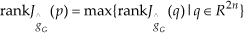
where J_ĝG (p) is the Jacobian matrix of ĝG and J_ĝG(p) has the same form as the rigidity matrix R.

Definition 2.2 [12] Point p is a regular point of graph G with n vertices if

rank J_{{\overset{\land}{g}}_{G}} (p) = \max {rank J_{{\overset{\land}{g}}_{G}} (q) | q \in R^{2 n}}

(7)

Lemma 2.1[26, 27] A framework (G,p) is infinitesimally rigid if and only if (G,p) is rigid and p is a regular point.

Lemma 2.1 tells us that some frameworks are rigid but not infinitesimally rigid. However, if the framework is infinitesimally rigid, then it is sure to be rigid. Fig. 1 illustrates these properties with two examples. It is easy to compute that rankJ_ĝG(q)=2n−3 in Fig. 1 (a) and rankJ_ĝG(q)<2n−3 in Fig. 1 (b), so Fig. 1 (a) is rigid and infinitesimally rigid; Fig. 1 (b) is rigid but not infinitesimally rigid as p is not a regular point. In general, the rigid graphs which fail to be infinitesimally rigid almost have parallel or collinear edges. In this paper, “rigid” almost always means “infinitesimally rigid”.

Figure 1.

Two possible examples with a rigid framework

Lemma 2.2 [28] Consider a formation F in R² with agents in generic positions and with defined agent pairs having the inter-agent distances maintained. Let G = (V, E) be the undirected graph. Then F is rigid if and only if there is a subset E'⊆E satisfying the following two conditions:

|E′| = 2|V| × 3.

For all E″ ⊆ E′,E″ ≠ ø

|E″|<<2|V(E″)|−3, where |V(E″)| is the number of vertices which are the end vertices of the edges in E″.

2.2 Persistent and minimally persistent graph

Rigidity is the property of the undirected graph, and persistence is the corresponding property of the directed graph.

Lemma 2.3 [15] A representation is persistent if and only if it is rigid and constraint consistent. A graph is generally persistent if and only if it is generally rigid and generally constraint consistent.

From Lemma 2.3, we know that rigidity and constraint consistence are the crucial factors for the persistence of a directed graph. However, in the plane, the rigidity of a directed graph is actually the rigidity of the corresponding underlying undirected graph, and the constraint consistence means that every agent should satisfy all their own distance constraints.

As a result, the graph in Fig.2 (a) is persistent and the graph in Fig.2 (b) is not persistent as node 2 is not constraint consistent (one node is able to satisfy two distance constraints at most in the plane). The arrows in the figures indicate the “leading” relationship, instead of the direction of the information flow which is commonly used in graph persistent theory [14]. As a result, the arrows indicating node 4 in Fig.2 (a) mean that node 4 is the “leader” of node 1, 2 and 3; node 1, 2 and 3 can only know the information of node 4.

Figure 2.

Example of a persistent and not persistent graph, (a) A graph is rigid and persistent; (b) A graph is rigid but not persistent

The minimal rigid graph requires that the graph has the least edges to satisfy the rigid conditions, and if one edge is removed, the graph will not be rigid. A comparative relationship between the rigidity and persistence is that the conditions of the minimally persistent graph are more complicated than that of the rigidity graph.

Lemma 2.4 [15] Consider a directed graph with more than one vertex. Then it is minimally persistent if and only if the underlying undirected graph is minimally rigid and no vertex has more than two outgoing edges.

Lemma 2.3 and Lemma 2.4 tell us that the number of the vertices in a minimally persistent graph is always 2n−3 (n represents the number of nodes).

3. Formation control laws

An example of minimally persistent formation with three co-leaders is shown in Fig 3 in which agent 4, 5 and 6 are the leaders in a cycle and each of them has one Degree of Freedom (DF). The DF of any of the followers 1, 2 and 3 is zero. All the followers are directly or indirectly controlled by the leaders to fulfil the distance constraint, i.e., the motion of agent 1 is constrained by agents 4 and 6; while the motion of agent 2 is constrained by agent 4 and agent 1.

Figure 3.

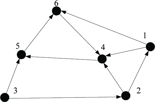
A graph with a minimally persistent formation with three co-leaders.

In this paper, the first order kinematic model is adopted for every agent:

u_{i} = \overset{\cdot}{p_{i}}

(8)

3.1 Control laws for followers

For n agents, the index of all the followers is defined from 1 to n-3. When one agent p_i has to maintain the constant distance (d_{ij_0} and d_{ik_0}) from two leader neighbours (p_j and p_k), it has two choices (shown in Fig. 4). Agent p_i may choose p_{i_0} or p_{i_0} as its targeted position since both of them have “the same distance (d_{ij_0} and d_{ik_0}) to p_j and p_k. However, the position p_{i_0} is more feasible than p′_{i_o} due to a short moving distance. Therefore, p_{i_0} is chosen as the target position to be reached for” the follower agent p_i. All the followers in this paper are guided by such a principle.

Figure 4.

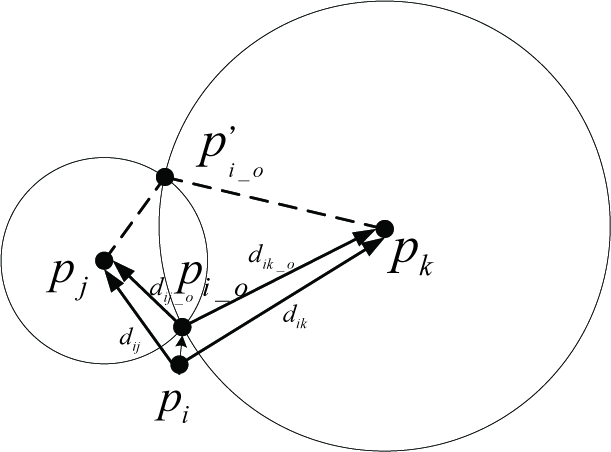
Moving principle of the followers.

From (8), we can design the control law:

\begin{array}{l} u_{i} = \overset{\cdot}{p_{i}} = K_{i} (p_{i_o} - p_{i}) \\ = K_{i} f (p_{j} - p_{i}, p_{k} - p_{i}, d_{i j_o}, d_{i k_o}) \end{array}

(9)

where K_i is the gain here.

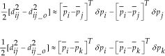
Suppose that the position of agent p_i can be expressed as p_i(t)=p̄ _i +δp_i(t), where p̄ _i (p̄ _i =(x̄ _i ,ȳ _i )) is the desired position which satisfies the dynamic constraint on the distance for the ith agent, and δp_i (t) means a small variable. From Fig.4, by using the cosine law to the triangle pipjp_{i_0} and neglecting the non-linear second order terms, a linear equation can be obtained as follows:

2 [{\bar{x}}_{j} - {\bar{x}}_{i} {{\bar{y}}_{j} - {\bar{y}}_{i}]}^{T} (p_{i_o} - p_{i}) \approx d_{i j}^{2} - d_{i j_o}^{2}

(10)

where d_ij represents the distance between p_i and p_j, and d_{ij_o} means the distance between p_i and p_{i_o}.

p_{i_o} - p_{i} \approx \frac{1}{2} {[\begin{array}{l} {\bar{x}}_{j} - {\bar{x}}_{i} {\bar{y}}_{j} - {\bar{y}}_{i} \\ {\bar{x}}_{k} - {\bar{x}}_{i} {\bar{y}}_{k} - {\bar{y}}_{i} \end{array}]}^{- 1} [\begin{array}{l} d_{i j}^{2} - d_{i j_o}^{2} \\ d_{i k}^{2} - d_{i k_o}^{2} \end{array}]

Then,

\begin{array}{l} \frac{1}{2} [d_{i j}^{2} - d_{i j_o}^{2}] \approx {[{\bar{p}}_{i} - {\bar{p}}_{j}]}^{T} δ p_{i} - {[{\bar{p}}_{i} - {\bar{p}}_{j}]}^{T} δ p_{j} \\ \frac{1}{2} [d_{i j}^{2} - d_{i j_o}^{2}] \approx {[{\bar{p}}_{i} - {\bar{p}}_{k}]}^{T} δ p_{i} - {[{\bar{p}}_{i} - {\bar{p}}_{k}]}^{T} δ p_{k} \end{array}

As a result, the control law of the followers is represented by:

[\begin{array}{l} \overset{\cdot}{δ x_{i}} \\ \overset{\cdot}{δ y_{i}} \end{array}] = K_{i} [\begin{array}{l} {\bar{x}}_{j} - {\bar{x}}_{i} \\ {\bar{x}}_{k} - {\bar{x}}_{i} \end{array} {\begin{array}{l} {\bar{y}}_{j} - {\bar{y}}_{i} \\ {\bar{y}}_{k} - {\bar{y}}_{i} \end{array}]}^{- 1} R_{(i j, i k)} [\begin{array}{l} δ x_{i} \\ δ y_{i} \\ δ x_{j} \\ δ y_{j} \\ δ x_{k} \\ δ y_{k} \end{array}]

(11)

\begin{aligned} R_{(i j, i k)} = & [\begin{matrix} {\bar{x}}_{i} - {\bar{x}}_{j} & {\bar{y}}_{i} - {\bar{y}}_{j} & - {\bar{x}}_{i} + {\bar{x}}_{j} & - {\bar{y}}_{i} + {\bar{y}}_{j} \\ {\bar{x}}_{i} - {\bar{x}}_{k} & {\bar{y}}_{i} - {\bar{y}}_{k} & 0 & 0 \end{matrix} ​ \\ ​ \begin{matrix} 0 & 0 \\ - {\bar{x}}_{i} + {\bar{x}}_{k} & - {\bar{x}}_{i} + {\bar{x}}_{k} \end{matrix}] \end{aligned}

(12)

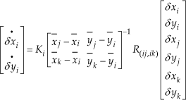
where R_(ij_,ik) is the sub-matrix of the rigidity matrix R. (Please see [17] for more details).

So, for all the followers, the control law can be obtained as follows:

\begin{array}{l} \overset{\cdot}{δ p (t)} = K R_{e}^{- 1} R δ p (t) \\ R_{e} = [\begin{array}{l} {\bar{x}}_{j} - {\bar{x}}_{i} \\ {\bar{x}}_{k} - {\bar{x}}_{i} \end{array} \begin{array}{l} {\bar{y}}_{j} - {\bar{y}}_{i} \\ {\bar{y}}_{k} - {\bar{y}}_{i} \end{array}] \end{array}

(13)

where both K and R_e are 2×2 diagonal block matrices. R_e partly represents the rigidity of the formation.

3.2 Control laws for co-leaders

There are three co-leaders indexed by n-2, n-1, and n, and they lead each other. The minimally persistent formation controllers for three co-leaders are proposed as:

\begin{array}{l} \overset{\cdot}{p_{n - 2}} = k_{n - 2} \frac{| | p_{n - 1} - p_{n - 2} | | - d_{(n - 2, n - 1)_o}}{| | p_{n - 1} - p_{n - 2} | |} (p_{n - 1} - p_{n - 2}) \\ \overset{\cdot}{p_{n - 1}} = k_{n - 1} \frac{| | p_{n} - p_{n - 1} | | - d_{(n - 1, n)_o}}{| | p_{n} - p_{n - 1} | |} (p_{n} - p_{n - 1}) \\ \overset{\cdot}{p_{n}} = k_{n} \frac{| | p_{n - 2} - p_{n} | | - d_{(n, n - 2)_o}}{| | p_{n - 2} - p_{n} | |} (p_{n - 2} - p_{n}) \end{array}

(14)

where k_n, k_n-1 and k_n_₂ are the gains.

Then

[\begin{array}{l} \overset{\cdot}{δ x_{n - 2}} \\ \overset{\cdot}{δ y_{n - 2}} \end{array}] = k_{n - 2} I_{2} R_{e_n - 2}^{- 1} R_{((n - 2) (n - 1), 00)} [\begin{array}{l} δ x_{n - 2} \\ δ y_{n - 2} \\ δ x_{n - 1} \\ δ y_{n - 1} \end{array}]

(15)

where

\begin{aligned} R_{((n - 2) (n - 1), 00)} = [\begin{matrix} {\bar{x}}_{n - 2} - {\bar{x}}_{n - 1} & {\bar{y}}_{n - 2} - {\bar{y}}_{n - 1} \\ 0 & 0 \end{matrix} ​ \\ ​ \begin{matrix} {\bar{x}}_{n - 1} - {\bar{x}}_{n - 2} & {\bar{y}}_{n - 1} - {\bar{y}}_{n - 2} \\ 0 & 0 \end{matrix}] \end{aligned}

(16)

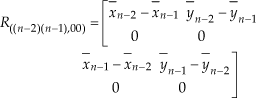
R_{e_n_}₂ is the sub-matrix of R_e corresponding to node n-2. Refer to (10), the R_{e_n_2} becomes:

R_{e_n - 2} = [\begin{matrix} {\bar{x}}_{n - 1} - {\bar{x}}_{n - 2} & {\bar{y}}_{n - 1} - {\bar{y}}_{n - 2} \\ - ({\bar{y}}_{n - 1} - {\bar{y}}_{n - 2}) & - ({\bar{x}}_{n - 1} - {\bar{x}}_{n - 2}) \end{matrix}]

(17)

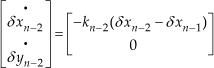
Each row of R_{e_n_}₂ is derived based on (10). As a result, the control law for p_n_₂ is:

\overset{\cdot}{δ p_{n - 2} (t)} = k_{n - 2} I_{2} R_{e_n - 2}^{-1} R_{((n - 2) (n - 1), 00)} δ p_{n - 2} (t)

(18)

Similarly, we get:

\overset{\cdot}{δ p_{n - 1} (t)} = k_{n - 1} I_{2} R_{e_n - 1}^{-1} R_{((n - 1) n, 00)} δ p_{n - 1} (t)

(19)

where

\begin{array}{l} R_{((n - 1) n, 00)} = [\begin{matrix} {\bar{x}}_{n - 1} - {\bar{x}}_{n} & {\bar{y}}_{n - 1} - {\bar{y}}_{n} \\ 0 & 0 \end{matrix} ​ \\ ​ \begin{matrix} {\bar{x}}_{n} - {\bar{x}}_{n - 1} & {\bar{y}}_{n} - {\bar{y}}_{n - 1} \\ 0 & 0 \end{matrix}] \\ R_{e_n - 1} = [\begin{matrix} {\bar{x}}_{n} - {\bar{x}}_{n - 1} & {\bar{y}}_{n} - {\bar{y}}_{n - 1} \\ - ({\bar{y}}_{n} - {\bar{y}}_{n - 1}) & - ({\bar{x}}_{n} - {\bar{n}}_{n - 1}) \end{matrix}] \end{array}

and

\begin{array}{l} δ \dot{p_{n}} (t) = k_{n} I_{2} R_{e_n}^{1} R_{(n (n - 2), 00)} δ_{p_{n}} (t) \\ R_{(n (n - 2), 00)} = [\begin{matrix} {\bar{x}}_{n} - {\bar{x}}_{n - 2} & {\bar{y}}_{n} - {\bar{y}}_{n - 2} \\ 0 & 0 \end{matrix} ​ \\ ​ \begin{matrix} {\bar{x}}_{n - 2} - {\bar{x}}_{n} & {\bar{y}}_{n - 2} - {\bar{y}}_{n} \\ 0 & 0 \end{matrix}] \\ R_{e_n} = [\begin{matrix} {\bar{x}}_{n - 2} - {\bar{x}}_{n} & {\bar{y}}_{n - 2} - {\bar{y}}_{n} \\ - ({\bar{y}}_{n - 2} - {\bar{y}}_{n}) & - ({\bar{x}}_{n - 2} - {\bar{x}}_{n}) \end{matrix}] \end{array}

(20)

3.3 Control laws for the whole formation

Without loss of generality, any 2D linear motion can be equivalent to a two-step motion consisting of translation along the x-axis and y-axis. To simplify the analysis process, a two-step translation along the x-axis and y-axis are used to substitute the linear motion in this paper.

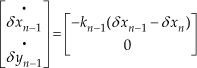
For the first step of the translation along the x-axis, the leader who firstly discovers the goal is defined as node n. In order to realize the x-axis translation, let the values of δy_n,δx_n,δy_n−1 and δy_n−2 all be zero, hence the values of ȳ_n−2 - ȳ_n−1, ȳ _n −ȳ_n−1 and ȳ_n−2−ȳ _n are also zero.

So we get that:

[\begin{array}{l} \overset{\cdot}{δ x_{n - 2}} \\ \overset{\cdot}{δ y_{n - 2}} \end{array}] = [\begin{matrix} - k_{n - 2} (δ x_{n - 2} - δ x_{n - 1}) \\ 0 \end{matrix}]

(21)

[\begin{array}{l} \overset{\cdot}{δ x_{n - 1}} \\ \overset{\cdot}{δ y_{n - 1}} \end{array}] = [\begin{matrix} - k_{n - 1} (δ x_{n - 1} - δ x_{n}) \\ 0 \end{matrix}]

(22)

[\begin{array}{l} \overset{\cdot}{δ x_{n}} \\ \overset{\cdot}{δ y_{n}} \end{array}] = 0

(23)

Likewise, for the second step of the translation along the y-axis, we arrive at the following conclusion:

[\begin{array}{l} \overset{\cdot}{δ x_{n - 2}} \\ \overset{\cdot}{δ y_{n - 2}} \end{array}] = [\begin{matrix} 0 \\ - k_{n - 2} (δ y_{n - 2} - δ y_{n - 1}) \end{matrix}]

(24)

[\begin{array}{l} \overset{\cdot}{δ x_{n - 1}} \\ \overset{\cdot}{δ y_{n - 1}} \end{array}] = [\begin{matrix} 0 \\ - k_{n - 1} (δ y_{n - 1} - δ y_{n - 2}) \end{matrix}]

(25)

[\begin{array}{l} \overset{\cdot}{δ x_{n}} \\ \overset{\cdot}{δ y_{n}} \end{array}] = 0

(26)

Since the translation along the x-axis and y-axis is equivalent, we can only discuss the case of translation along the x-axis here.

With (11), (21), (22) and (23), we obtain a new control law:

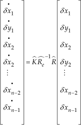
[\begin{array}{l} \overset{\cdot}{δ x_{1}} \\ \overset{\cdot}{δ y_{1}} \\ \overset{\cdot}{δ x_{2}} \\ \overset{\cdot}{δ x_{2}} \\ ⋮ \\ \overset{\cdot}{δ x_{n - 2}} \\ \overset{\cdot}{δ x_{n - 1}} \end{array}] = \hat{K} {\hat{R_{e}}}^{- 1} \hat{R} [\begin{array}{l} \overset{​}{δ x_{1}} \\ \overset{​}{δ y_{1}} \\ \overset{​}{δ x_{2}} \\ \overset{​}{δ y_{2}} \\ ⋮ \\ \overset{​}{δ x_{n - 2}} \\ \overset{​}{δ x_{n - 1}} \end{array}]

(27)

where $\hat{K} = (\oplus_{i = 1}^{n - 3} K_{i}) \oplus k_{n - 2} \oplus k_{n - 1}$

The number of the rest control variable is only (2n−4) since δy_n,δx_n,δy_n−1 and δy_n−2 are all zero, so both R_e and R are (2n−4)×(2n−4). As R is originally (2n−3)x2n (2n−4), (2n−2), (2n−1), 2n columns and the (2n−2) row will be removed from R to get R because they are corresponding to the zero value of δy_n,δx_n,δy_n−1 and δy_n−2. Based on the same reason, R⌢_e is derived by removing (2n−4), (2n−2), (2n−1) and 2n columns fromR_e.

Then the set of all the follower nodes is denoted by V and a subset of the follower node set is V′_f,V′_f ⊂ V′.

\hat{R} = [\begin{matrix} R (V^{'}) & ​ & X & ​ \\ 0 & {\bar{x}}_{n - 2} - {\bar{x}}_{n - 1} & {\bar{x}}_{n - 1} - {\bar{x}}_{n - 2} & 0 \\ 0 & {\bar{x}}_{n - 2} - {\bar{x}}_{n} & 0 & {\bar{x}}_{n} - {\bar{x}}_{n - 2} \end{matrix}]

(28)

\hat{R_{e}} = (\oplus_{i = 1}^{n - 3} D_{i}) \oplus (x_{n - 1} - x_{n - 2}) \oplus (x_{n} - x_{n - 1})

(29)

Here, we suppose that the two outgoing edges from node i are {p_i, p_j}and{p_i, p_k}, so:

D_{i} = - [\begin{matrix} x_{i} - x_{j} & y_{i} - y_{j} \\ x_{i} - x_{k} & y_{i} - y_{k} \end{matrix}]

(30)

4. Stability analysis

In section 3, we propose the formation control laws using the minimally persistent directed graph. In this section the stability of the control laws will be discussed.

The control laws will be expressed by:

\overset{\cdot}{z} = \hat{K} {\hat{R_{e}}}^{- 1} \hat{R} z

Where $\hat{K} {\hat{R_{e}}}^{- 1}$ can be expressed by $\hat{K_{Re}}$ and $\hat{K_{Re}}$ is a diagonal block matrix. Then the above equation is easily transformed into:

\overset{\cdot}{z} = \hat{K_{Re}} \hat{R} z

(31)

Theorem 4.1 For an n-node minimally persistent formation with the agent set P = {p₁,p₂,…,p_n} at generic positions, the three co-leaders are indexed by n, n-1 and n-2. R is the matrix obtained by removing the (2n−4), (2n−2), (2n−1) and 2n columns, and (2n−2) row, from the rigidity matrix R. Then a diagonal block matrix K _Re exists, such that the formation control laws (31) with the minimally persistent are stable.

Proof. In Theorem 3.2 in [17], we obtain the conclusion that if every leading principal minor of R̂ is nonzero, then a diagonal A exists such that the real parts of the eigenvalues of ΛR̂ are all negative.

Following Lemma 4.3 and Theorem 4.5 in [17], we know that both R(V') and R(V′_f) are generally non-singular (V′_f⊂V′) with one leader formation.

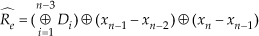
Finally, for all 1 ≤ k ≤ n-3, the outgoing edges from the vertex k are the main factor of R̂, so with the leading principal minor of R(V_f), there are three situations to be considered here.

The leading principal minor of R̂ is denoted by D_i {i = 1,2,3 n−l}. On account of the sequence appearing in the leading principal minor, only the last appearing node needs to be considered here. Suppose that the last appearing node is p_k, and its virtual leaders are p_m,p_n. The edges from p_k are{p_k,p_m} and {p_k,p_n}.

If m < k and n < k, which means that the index of both p_m and p_n are smaller than that of p_k in the sequence of the leading principal minor, then this leading principal minor is |R(V′_f)|. As analysed in [17], it is known that R(V′_f) is non-singular, so the determinant here is nonzero.

If (m<k<n) or (n<k<m). For the case of (m<k<n), when both of p_m,p_n. are the followers, and as R(V_f) is non-singular, so the determinant is nonzero; when p_n is the co-leader, from Lemma 4.3 and Theorem 4.5 in [17], it is known that the determinant is also nonzero

If m > kandn > k, there are three situations that need to be discussed.

When both of them are followers, then it is similar to step (1); when one of them is the follower and the other is a co-leader, then it is similar to step (2); when both of them are co-leaders, then the leading principal minor is:

D_{k} = \det ([\begin{matrix} R (1, 2, 3, &, k - 1) & ​ & X \\ 0 & {\bar{x}}_{k} - {\bar{x}}_{m} & {\bar{y}}_{k} - {\bar{y}}_{m} \\ 0 & {\bar{x}}_{k} - {\bar{x}}_{n} & {\bar{y}}_{k} - {\bar{y}}_{m} \end{matrix}])

where X is a don't-care vector and x̄, ȳ are the x-axis and y-axis coordinates. So it is also nonzero.

To sum up, the leading principal minor of all the followers is nonzero. Then the leading principal minor of the co-leaders is provided as follows:

\begin{array}{l} D_{2 n -5} = \det ([\begin{matrix} R (V^{'}) & ​ & X \\ 0 & {\bar{x}}_{n - 2} - {\bar{x}}_{n - 1} & {\bar{x}}_{n - 1} - {\bar{x}}_{n - 2} \end{matrix}]) \\ D_{2 n - 4} = \det ([\begin{matrix} R (V^{'}) & ​ & X & ​ \\ 0 & {\bar{x}}_{n - 2} - {\bar{x}}_{n - 1} & {\bar{x}}_{n - 1} - {\bar{x}}_{n - 2} & 0 \\ 0 & {\bar{x}}_{n - 2} - {\bar{x}}_{n} & 0 & {\bar{x}}_{n} - {\bar{x}}_{n - 2} \end{matrix}]) \end{array}

Both of them can be transformed into the form as follows:

\tilde{D} = \det ([\begin{matrix} R (1, 2, 3, &, n - 3) & X \\ 0 & \bar{k} \bar{x} \end{matrix}])

where k̄ is the real coefficient gain and x indicates the real number, such as x̄_n−1,x̄_n−2 and x̄_n. As a result, they are nonzero.

Therefore, the leading principal minor of $\hat{R}$ is nonzero. From Theorem 3.2 in reference [17], we know that a diagonal $\hat{K_{Re}}$ exists such that the real parts of the eigenvalues of (31) are all negative, Theorem 4.1 holds.

5. Simulations

In this section, simulations using the control laws designed in this paper are presented. Mobilesim software is used to conduct the simulation platforms.

In the simulations, the topology of the mobile robot system is the same as in Fig. 3, in which robots 4, 5 and 6 are defined as the leaders, and the others are the followers.

As analysed in section 3.3, to simplify the analysis, the simulations consist of two stages which are moving along the x-axis and then along the y-axis. In addition, two kinds of follower topology are studied, which are cyclic and acyclic.

In Fig.5 (a), the topology of the leader set {4,5,6} is cyclic and the topology of the follower set {1,2,3} is acyclic.

Figure 5.

Simulation snapshots for a three co-leader minimally persistent formation with followers in an acyclic graph.

In the simulations, the gains applied in the controller are defined as follows:

{\hat{R_{e}}}^{- 1} \hat{R} = [\begin{matrix} S (V^{'}) & X \\ 0 & S_{L} \end{matrix}]

where

S_{L} = [\begin{matrix} - 1 & 1 & 0 \\ 0 & - 1 & 1 \end{matrix}]

Node {1,2,3}⊂V′, and their topology is acyclic, so based on Theorem 5.2 in [17], we know that all the eigenvalues corresponding to node {1,2,3} are −1. So only the eigenvalues corresponding to the leader needed to be adjusted by k̂.

\hat{K} = [\begin{matrix} 1 & 0 & 0 & 0 & 0 & 0 & 0 & 0 \\ 0 & 1 & 0 & 0 & 0 & 0 & 0 & 0 \\ 0 & 0 & 1 & 0 & 0 & 0 & 0 & 0 \\ 0 & 0 & 0 & 1 & 0 & 0 & 0 & 0 \\ 0 & 0 & 0 & 0 & 1 & 0 & 0 & 0 \\ 0 & 0 & 0 & 0 & 0 & 1 & 0 & 0 \\ 0 & 0 & 0 & 0 & 0 & 0 & k_{n - 2} & 0 \\ 0 & 0 & 0 & 0 & 0 & 0 & 0 & k_{n - 1} \end{matrix}]

Snapshot (a) and (b) in Fig. 5 show that the formation is moving with the following initial position:

\begin{array}{l} p_{1} = (3.8, 1.0), p_{2} = (- 1.4, 1.8), \\ p_{3} = (0.5, 5.8), p_{4} = (2.2, 2.5), \\ p_{5} = (3.5, 5.4), p_{6} = (5.1, 4.2) . \end{array}

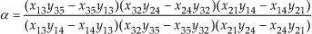
Considering the property of ${\hat{R_{e}}}^{- 1} \hat{R}$ , here we may choose $k_{n - 2} = k_{n - 1} = - 1$ . Fig.5 (c) depicts that the robots have adjusted their orientation along the y-axis. In Fig.5 (d), all the robots finally arrive at the destination.

Then, another situation is considered where the topology of the follower set {1,2,3} is cyclic. The snapshots are shown in Fig 6.

Figure 6.

Simulation snapshots for a three co-leader minimally persistent formation with followers in a cyclic graph.

The initial positions of the robots are defined as follows:

\begin{array}{l} p_{1} = (- 2.5, 5.7), p_{2} = (- 6.3, 3.8), \\ p_{3} = (- 2.8, 11.6), p_{4} = (- 1.2, 3.6), \\ p_{5} = (2.8, 10.1), p_{6} = (5.6, 8.8) . \end{array}

Both the leaders and followers are in a cycle, hence it is more complex than the first situation.

From [17], we know that: if the topology of V′_f={1,…,k}⊂V′ is cyclic, define a to be the trace of the cycle weight. Then k eigenvalues of S(V′) are at −1, and the remaining are at $- 1 + α^{\frac{1}{k}} e^{\frac{2 π l}{k}}, l \in {0, \dots, k - 1}$ , where α is defined as:

α = \frac{(x_{13} y_{35} - x_{35} y_{13}) (x_{32} y_{24} - x_{24} y_{32}) (x_{21} y_{14} - x_{14} y_{21})}{(x_{13} y_{14} - x_{14} y_{13}) (x_{32} y_{35} - x_{35} y_{32}) (x_{21} y_{24} - x_{24} y_{21})}

For this designed persistent formation (k=3), the eigenvalues for S(V') are:

\begin{matrix} - 1, - 1, - 1, - 0.380 0 + 1.073 9 i, \\ 4.035 2 + 8.721 2 i, 39, 888 9 + 70.821 7 i \end{matrix}

K̂ is chosen as follows:

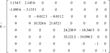
\hat{K} = [\begin{matrix} 1.1345 & 2.1456 & 0 & 0 & 0 & 0 & 0 & 0 \\ - 1.0986 & - 3.1351 & 0 & 0 & 0 & 0 & 0 & 0 \\ 0 & 0 & - 0.0123 & - 0.0112 & 0 & 0 & 0 & 0 \\ 0 & 0 & 10.3246 & 21.6521 & 0 & 0 & 0 & 0 \\ 0 & 0 & 0 & 0 & 24.2389 & - 18.3465 & 0 & 0 \\ 0 & 0 & 0 & 0 & 33.1212 & - 19.0982 & 0 & 0 \\ 0 & 0 & 0 & 0 & 0 & 0 & - 1 & 0 \\ 0 & 0 & 0 & 0 & 0 & 0 & 0 & - 1 \end{matrix}]

The eigenvalues of $\hat{k} {\hat{R}}_{e}^{- 1} \hat{R}$ are:

\begin{array}{l} {- 1.000 0, - 1.000 0, \\ - 0.283 5 - 0.483 2 i, \\ - 21.8592 - 0.387 9 i, \\ - 2.570 4 + 11.753 0 i, \\ - 2.570 3 - 11.753 0 i, \\ - 12.925 2 - 26.539 8 i, \\ - 0.156 7 + 0.416 3 i} \end{array}

So it can be proved that this situation is also stable.

6. Conclusions

This paper mainly dealt with the problem of minimally persistent formation control with three co-leaders, and the minimally persistent formation control law for the case where three co-leaders are in the cycle was proposed. The non-square matrix, which mostly represents the characteristic of the persistent formation, is successfully utilized to design the control law. In the process of designing the control laws, the straight line motion is substituted by a two-step translation motion along the x-axis and y-axis, respectively. The method of leading principal minor is adopted to prove that the system with the designed law can be stabilized. The simulation results demonstrate that whether or not the followers lie on a cyclic graph, the designed control law is effective.

Footnotes

7. Acknowledgments

The authors would like to thank the Editor-in-Chief, the Associate Editor, and anonymous reviewers for their constructive suggestions to improve the quality of this paper. This work was supported by the Projects of Major International (Regional) Joint Research Program NSFC (61120106010), National Science Fund for Distinguished Young Scholars No. (60925011), NSFC (61175112), and Beijing bionic robot and system the key laboratory.

References

Olfati-Saber

Murray

. Distributed cooperative control of multiple vehicle formations using structural potential functions. Proc. of 15th IFAC World Congress, 2002: 1–7.

Olfati-Saber

Dunbar

Murray

Cooperative control of multi-vehicle systems using cost graphs and optimization. Proc. of American Control Conference, 2003: 2217–2222.

Tanner

H G

Jadbabaie

Pappas

G J.

Stable flocking of mobile agents, part I: Fixed topology. Proc. of 42nd IEEE Conference on Decision and Control, 2003: 2010–2015.

Tanner

H G

Jadbabaie

Pappas

G J.

Stable flocking of mobile agents part II: Dynamic topology. Proc. of 42nd IEEE Conference on Decision and Control, 2003: 2016–2021.

Sorensen

Wei

A unified formation control scheme with a single or multiple leaders. Proc. of American Control Conference. ACC '07, 2007: 5412–5418.

Krick

Broucke

M E

Francis

B A.

Stabilization of infinitesimally rigid formations of multi-robot networks. Proc. of 47th IEEE Conference on Decision and Control. CDC 2008, 2008: 477–482.

Tran

Lee

A stable formation control using approximation of translational and angular accelerations. International Journal of Advanced Robotic Systems, 2011, 8(1): 65–75.

Jiang

Zhang

Stable formation control of multi-robot system with communication delay. International Journal of Advanced Robotic Systems, 2012, 9(4).

Oscar

Patricia

Intelligent adaptive model-based control of robotic dynamic systems with a hybrid fuzzy-neural approach. Applied Soft Computing, 2003, 3(4): 363–378.

10.

Leocundo

Patricia

Oscar

Intelligent control of a stepping motor drive using a hybrid neuro-fuzzy ANFIS approach. Applied Soft Computing, 2003, 3(3): 363–378.

11.

Eren

Anderson

B D O

Morse

A S

Operations on rigid formations of autonomous agents. Communications in Information and Systems, 2004, 4(3): 209–219.

12.

Krick

Broucke

M E

Francis

B A.

Stabilization of infinitesimally rigid formations of multi-robot networks. Proc. of 47th IEEE Conference on Decision and Control. CDC 2008, 2008: 477–482.

13.

Tay

Whiteley

Generating isostatic frameworks. Structural Topology, 1985, 11: 21–69.

14.

Hendrickx

J M

Anderson

B D O

Blondel

V D.

Rigidity and persistence of directed graphs. Proc. of 44th IEEE Conference on Decision and Control and 2005 European Control Conference. CDC-ECC '05, 2005: 2176–2181.

15.

Hendrickx

J M

Anderson

B D O

Delvenne

Directed graphs for the analysis of rigidity and persistence in autonomous agent systems. International Journal Of Robust And Nonlinear Control, 2007, 17(10–11): 960–981.

16.

Hendrickx

J M

Fidan

Changbin

Formation reorganization by primitive operations on directed graphs. Automatic Control, IEEE Transactions on, 2008, 53(4): 968–979.

17.

Anderson

B D O

Dasgupta

Control of minimally persistent formations in the plane. Siam Journal On Control And Optimization, 2009, 48(1): 206–233.

18.

Tabuada

Pappas

G J

Lima

Cyclic directed formations of multi-agent systems. Proc. of 40th IEEE Conference on Decision and Control, 2001: 56–61.

19.

Baillieul

Suri

Information patterns and hedging Brockett's theorem controlling vehicle formations. Proc. of 42nd IEEE Conference on Decision and Control, 2003: 556–563.

20.

Anderson

B D O.

Development of redundant rigidity theory for formation control. International Journal of Robust and Nonlinear Control, 2009, 19(13): 1427–1446.

21.

Fidan

Hendrickx

J M

Anderson

B D O.

Closing ranks in rigid multi-agent formations using edge contractions. International Journal of Robust and Nonlinear Control, 2010, 20(18): 2077–2092.

22.

Cao

Morse

A S

Anderson

B D O

Dasgupta

. Maintaining a directed, triangular formation of mobile autonomous agents. Communications in Information and Systems (special issue honouring John Bailleul), 2011, 11(1): 1–16.

23.

Motevallian

S A

Anderson

B D O.

Multi-agent rigid formations: A study of robustness to the loss of multiple agents. Proc of IEEE Conference on Decision and Control and European Control Conference, 2011: 3602–3607.

24.

Marshall

J A

Broucke

M E

Francis

B A.

Formations of vehicles in cyclic pursuit. Automatic Control, IEEE Transactions on, 2004, 49(11): 1963–1974.

25.

Anderson

B D O

Dasgupta

Control of a three-coleader formation in the plane. Systems & Control Letters, 2007, 56(9–10): 573–578.

26.

Asimow

Roth

Rigidity of graphs. Transactions of the American Mathematical Society, 1978(245): 279–289.

27.

Asimow

Roth

The rigidity of graphs, II. Journal of Mathematical Analysis and Applications, 1979, 1(68): 171–190.

28.

Laman

On graphs and the rigidity of plane skeletal structures. Journal of Engineering Mathematics, 1970(4): 331–340.

Control of 2D Minimally Persistent Formations with Three Co-Leaders in a Cycle

Abstract

Keywords

1. Introduction

2. Preliminaries

2.1 Graph rigidity

2.2 Persistent and minimally persistent graph

3. Formation control laws

3.1 Control laws for followers

3.2 Control laws for co-leaders

3.3 Control laws for the whole formation

4. Stability analysis

5. Simulations

6. Conclusions

Footnotes

7. Acknowledgments

References