Sage Journals: Discover world-class research

Abstract

The mechanism with good fold performance derived from rigid origami is widely used in the field of engineering. In this article, the adjacency matrix method was proposed to analyze the degree of freedom of foldable plate rigid origami. This method can also judge the number of redundant constraints while calculating the degree of freedom of the rigid origami. First, the adjacency matrix between vertices of origami structure was established. Then the elimination matrix was introduced, and the process of determining the motion state of vertices was described by matrix product. The degree of freedom of rigid origami was determined by calculating the number of constraints introduced. A method for judging redundant constraints of rigid origami was proposed, and the number of redundant constraints was determined by computing the sum of the row elements corresponding to the vertices. The motion state of the cross-crease vertex was analyzed, and the computational error of the degree of freedom at the cross-crease vertex was avoided by the method of classification and simplification. The degree of freedom of the ring pattern was discussed, and the calculation method of the degree of freedom of whole pattern with many ring patterns was summarized. Finally, the degree of freedom of typical rigid origami was analyzed.

Keywords

Rigid origami degree of freedom calculation redundant constraint adjacency matrix origami pattern with multi-vertices

Introduction

The panels of rigid origami keep the rigidity in addition to creases, during the folding process. Many foldable mechanisms have been derived from rigid origami, which have the advantages of artful structure and is easy to fold. They have attracted wide attention and application in the field of practical engineering. In civilian areas, the mechanism derived from rigid origami can be used in the design of foldable dinnerware,¹ kayak,² shelter,³ and so on.^4–6 In the field of aerospace, the mechanism derived from rigid origami can be used in the design of the solar array.^7–9 In order to explore the principles of origami and develop more structures from rigid origami, more and more scholars are using mathematics to explain origami.

In the study of kinematics of origami, Kawasaki¹⁰ put forward the requirement of the angle between the creases when a single vertex can fold flat, thus becoming the basic theorems for flat-foldable origami with Maekawa’s¹¹ mountain-valley crease theory. Belcastro and Hull¹² modeled the paper using a matrix method, and discussed the necessary conditions of the rigid origami. Hull¹³ studied the influence of the mountain-valley assignment on flat foldability, discussed the sharp bounds of the distributions of the mountain-valley assignment in a flat vertex fold, and explored the analysis method of flat multiple vertex folds. Tachi¹⁴ built a fold simulation system for rigid origami models, and realized the fold simulation of some origami configurations, by triangulating the polygons and adjusting the crease lines. Wu and You¹⁵ established the motion model of origami by quaternions and dual quaternions, analyzed the flat foldability and rigid foldability of the initially flat or a non-flat pattern with a single vertex or multiple vertices, and judged the self-intersection of the origami in the folding process. Chen and Feng¹⁶ used a nonlinear algorithm to predict the folding behavior of the origami structure and present a numerical analysis and finite element simulation of the folding process. Abel et al.¹¹ proposed a necessary and sufficient condition for the rigid foldability of a single vertex, and laid the basic theory for the study of rigid origami. Chen et al.¹⁷ established a general kinematic model for rigid origami, obtained a series of deployable prismatic structures, and proposed a design method for single degree of freedom (DOF) multilayered prismatic structures. Cai et al.¹⁸ improved the quaternions method, verified the foldability of cylindrical origami configurations, and analyzed the motion of leaf pattern,¹⁹ Kresling pattern,^20,21 and cylinders with Miura-ori.²²

Several methods^23–25 have been proposed for the calculation of the DOF of the classical mechanism; however not many approaches are applicable to the DOF calculation of the rigid origami. In the study of DOF of the rigid origami, the empirical formula for calculating the DOF of rigid origami has been summarized.¹⁴ Cai et al.²⁶ established the system constraint equations using different constraints, and calculated the DOF of the rigid origami from the dimension of null space of the Jacobian matrix. However, the empirical formula of the DOF has some limitations. When the redundant constraints of the origami structure exist, the empirical formula of the DOF will not be applicable. The method proposed by Cai using the dimension of null space of the Jacobian matrix is complicated. When the origami pattern is sophisticated, the derivation of the null space of the Jacobian matrix can be too complex.

This article originally put forward a method to analyze the DOF of rigid origami by transforming the adjacency matrix. The adjacency matrix between vertices of origami is established and the required constraint of origami is determined by the transformation process of adjacency matrix. The DOF of rigid origami was determined by calculating the number of constraints introduced. It is superior to the empirical formula method that this method has applicability to the origami pattern with redundant constraints and can determine the number of redundant constraints and the location of redundant constraints in the analysis process. Compared with the method proposed by Cai, the calculation process of this method is simple and easy to be realized by computer programming.

In this article, the relation between the DOF and the number of edges of a single vertex is analyzed by screw theory, and then the adjacency matrix method is proposed to analyze the DOF of rigid origami with multi-vertices. The establishment of adjacency matrix, elimination transformation of matrix, calculation of DOF, and the judgment method of redundant constraint are introduced. Then two special cases are discussed. Finally, some examples are given to verify the correctness of the adjacency matrix method for analyzing the DOF of rigid origami with multi-vertices.

DOF of a single vertex

In kinematic analysis of rigid origami, the creases can be equivalent to revolute pairs, and the paper can be equivalent to the bar (as shown in Figure 1). In the analysis of the DOF of a single vertex, the motion screw system of the vertex is established using the screw theory,^27–30 and then the DOF of the single vertex is calculated by the modified G-K formula. In screw theory, the position of the coordinate system has no influence on the relevant and reciprocal relationship between the screws, so that the origin of the coordinate system can be chosen as the point at which the motion analysis is convenient. The vertex is chosen as the origin of the coordinate system. The direction of the crease 1 is the direction of the $x$ axis, the $y$ axis is normal to the $x$ axis, and the $z$ axis is determined by the right-hand rule.

Figure 1.

A single vertex equivalent to mechanism: (a) a vertex with m creases (m≧ 4) and (b) the equivalent mechanism of the vertex.

By analyzing the position of each rotating pair axis in the coordinate system $O - xyz$ , the corresponding screw system can be obtained. Since the rotation pairs are all at the same vertex which is the origin of the selected coordinate system, and then the position vector $r$ in the screw of the revolute pair $(S; r \times S)$ is $0$ , the dual unit $S_{0}$ in all the screw is $0$ , that is, $S_{0} = (0 0 0)$ . The kinematic screw system of a single vertex with $m$ creases is

{\begin{matrix} $_{1} = (1 0 0; 0 0 0) \\ $_{2} = (a_{2} b_{2} c_{2}; 0 0 0) \\ $_{3} = (a_{3} b_{3} c_{3}; 0 0 0) \\ $_{4} = (a_{4} b_{4} c_{4}; 0 0 0) \\ $_{5} = (a_{5} b_{5} c_{5}; 0 0 0) \\ ⋮ \\ $_{m} = (a_{m} b_{m} c_{m}; 0 0 0) \end{matrix}

(1)

The fourth to sixth elements in each screw are 0, indicating that there are at least three reciprocal screws for the kinematic screw system. Since a number of revolute pairs intersect at one point, there is a three-dimensional rotation in space, and the rank of the constraint screw system cannot be greater than 3. Based on the above analysis, we find that the constraint screw system of a single vertex is

{\begin{matrix} $_{1}^{r} = (1 0 0; 0 0 0) \\ $_{2}^{r} = (0 1 0; 0 0 0) \\ $_{3}^{r} = (0 0 1; 0 0 0) \end{matrix}

(2)

where $$_{1}^{r}$ , $$_{2}^{r}$ , and $$_{3}^{r}$ , respectively, indicate the binding force along the direction of the $x$ axis, the $y$ axis, and the $z$ axis, which limits the movement in the three-dimensional space.

Irrespective of the number of creases, a single vertex rigid origami always has a common binding force of three directions in space, so the rank of the equivalent mechanism $d$ is equal to 3. According to the modified G-K formula^31,32

M = d (n - g - 1) + \sum_{i = 1}^{g} f_{i} + v - ζ

(3)

where $M$ is the DOF of the mechanism, $d$ is the rank of the mechanism, $n$ is the number of components including the rack, $g$ is the number of kinematic pairs, $f_{i}$ represents the DOF of the kinematic pair $i$ , $v$ is the number of redundant constraints for multi-loop parallel mechanisms after removing common constraints, and $ζ$ is the local DOF in the mechanism. In analyzing the DOF of a single vertex rigid origami, $n$ is the number of faces between creases, $g$ is the number of creases, and all $f_{i}$ equals 1. There are no redundant constraints and local DOF in single vertex origami, so $v$ and $ζ$ are both 0.

For the vertex not at the boundary, there is still a connection between the rotation pair $$_{m}$ and $$_{1}$ , where the number of faces $n$ equals the number of creases $g$ , which is equal to $m$ , the number of edges at the vertices. Then the DOF of the vertex is^14,33

M = m - 3

(4)

For the boundary vertex, there is no face between $$_{1}$ and $$_{m}$ , and then $$_{1}$ and $$_{m}$ cannot be equivalent to revolute pairs. Then the face number $n$ is $m - 1$ , and the creases number $g$ is $m - 2$ . Equation (3) is no longer applicable, but each crease can be regarded as a revolute pair, and each revolute pair provides a rotational DOF. Then the total DOF of the vertex is

M = m - 2

(5)

DOF of the pattern with multi-vertices

In the previous section, the relation between the DOF of a vertex and the number of edges at the vertex is analyzed. It is easy to establish a kinematic screw system, as the relation between the positions of the creases in a single vertex is relatively simple. For multi-vertices, it is troublesome to analyze the DOF by establishing a kinematic screw system. The adjacency matrix method which is a simple method for calculating the DOF of rigid origami with multi-vertices is proposed here.

From the analysis of the previous section, it is shown that the DOF of the non-boundary vertex is equal to $m - 3$ , for example, the DOF of the vertex with four creases is 1, and the DOF of the vertex with five creases is 2; $m - 3$ constraints are provided for the vertex, and the motion of the vertex can be completely determined. In the deployable antenna pattern shown in Figure 2, the vertex 1 is a non-boundary vertex with five creases. According to equation (4), the DOF of vertex 1 is 2. When the rotation angle of any two creases is determined at the vertex 1, the rotation angle of the remaining three creases is also determined accordingly. Then the DOF of the vertex 2 is analyzed. The vertex 2 is also a non-boundary vertex with five creases, and the DOF of this vertex is 2. Since two constraints are added at the vertex 1, the rotation angle of the crease $l_{12}$ has been determined. At the vertex 2, only one more constraint is added, and the rotation angles of all the creases can be determined. The vertex 3 to the vertex 10 is the boundary vertex, and the DOF is calculated by equation (5). As for the deployable antenna pattern, when the rotation angles of the non-boundary vertices 1 and 2 are determined, the position of the boundary points is also determined. From the above analysis, we can see that the motion of deployable antenna will be completely determined after adding three non-redundant constraints, that is, the DOF of deployable antenna is 3.

Figure 2.

The simple model of the deployable antenna.

For patterns with many vertices, the above process of calculability will become tedious. Then this article proposed an adjacency matrix method to calculate the DOF of origami with multi-vertices. In the initial adjacency matrix $C_{0}$ of the origami pattern, “1” stands for two vertices connected with each other and “0” stands for two vertices that are not connected. Take the deployable antenna pattern shown in Figure 2 as an example, and the adjacency matrix is established as follows

C_{0} = \begin{matrix} \begin{matrix} 1 \\ 2 \\ 3 \\ 4 \\ 5 \\ 6 \\ 7 \\ 8 \\ 9 \\ 10 \end{matrix} & [\begin{matrix} 1 & 2 & 3 & 4 & 5 & 6 & 7 & 8 & 9 & 10 \\ 0 & 1 & 0 & 0 & 0 & 0 & 1 & 1 & 1 & 1 \\ 1 & 0 & 1 & 1 & 1 & 1 & 0 & 0 & 0 & 0 \\ 0 & 1 & 0 & 1 & 0 & 0 & 0 & 0 & 0 & 1 \\ 0 & 1 & 1 & 0 & 1 & 0 & 0 & 0 & 0 & 0 \\ 0 & 1 & 0 & 1 & 0 & 1 & 0 & 0 & 0 & 0 \\ 0 & 1 & 0 & 0 & 1 & 0 & 1 & 0 & 0 & 0 \\ 1 & 0 & 0 & 0 & 0 & 1 & 0 & 1 & 0 & 0 \\ 1 & 0 & 0 & 0 & 0 & 0 & 1 & 0 & 1 & 0 \\ 1 & 0 & 0 & 0 & 0 & 0 & 0 & 1 & 0 & 1 \\ 1 & 0 & 1 & 0 & 0 & 0 & 0 & 0 & 1 & 0 \end{matrix}] \end{matrix}

(6)

The number of “1s” in a row or column in the adjacency matrix $C_{0}$ represents the number of edges of corresponding vertex. For example, the first row of the matrix has 5 “1s,” and the vertex 1 has five edges. The relation between the number of edges and the DOF of the boundary vertices is different from that of the non-boundary vertices. When the vertices are numbered to establish the adjacency matrix, the non-boundary vertices are arranged before the boundary vertices, so as to facilitate the discussion of different types of vertices.

The variable $D$ is introduced to indicate the number of constraints required to determine the motion of the vertex. No constraints are added before analysis, and the motion of each vertex is undefined. In this case, $D_{0}$ is 0. According to equation (4), both the number of constraints required for vertices 1 and 2 are 2, then any vertex can be chosen as the minimum-constraint vertex to start the analysis, and now select vertex 1. The number of constraints required to determine the motion of vertex 1 is 2. After two constraints are provided for vertex 1, $D_{1}$ equals $D_{0} + 2$ . The motion at the vertex 1 is completely determined, and $C_{0}$ transforms into $C_{1}$

C_{1} = \begin{matrix} \begin{matrix} 1 \\ 2 \\ 3 \\ 4 \\ 5 \\ 6 \\ 7 \\ 8 \\ 9 \\ 10 \end{matrix} & [\begin{matrix} 1 & 2 & 3 & 4 & 5 & 6 & 7 & 8 & 9 & 10 \\ 0 & 0 & 0 & 0 & 0 & 0 & 0 & 0 & 0 & 0 \\ 0 & 0 & 1 & 1 & 1 & 1 & 0 & 0 & 0 & 0 \\ 0 & 1 & 0 & 1 & 0 & 0 & 0 & 0 & 0 & 1 \\ 0 & 1 & 1 & 0 & 1 & 0 & 0 & 0 & 0 & 0 \\ 0 & 1 & 0 & 1 & 0 & 1 & 0 & 0 & 0 & 0 \\ 0 & 1 & 0 & 0 & 1 & 0 & 1 & 0 & 0 & 0 \\ 0 & 0 & 0 & 0 & 0 & 1 & 0 & 1 & 0 & 0 \\ 0 & 0 & 0 & 0 & 0 & 0 & 1 & 0 & 1 & 0 \\ 0 & 0 & 0 & 0 & 0 & 0 & 0 & 1 & 0 & 1 \\ 0 & 0 & 1 & 0 & 0 & 0 & 0 & 0 & 1 & 0 \end{matrix}] \end{matrix}

(7)

In the matrix $C_{1}$ , the meaning of “1” changes, “1” indicates that the rotation angle of the corresponding crease is not given. The motion of each edge of the vertex 1 is determined, so the first row and first column of $C_{1}$ are changed to “0.” When the matrix $C_{0}$ is changed to $C_{1}$ , the elimination matrix $E_{j, n}$ is used. The elimination matrix is as follows

E_{j, n} = [\begin{matrix} 1 & 0 & \dots & 0 & 0 & \dots & 0 \\ 0 & 1 & \dots & 0 & 0 & \dots & 0 \\ ⋮ & ⋮ & ⋮ & ⋮ & ⋮ \\ 0 & 0 & \dots & 0_{j, j} & 0 & \dots & 0 \\ 0 & 0 & \dots & 0 & 1 & \dots & 0 \\ ⋮ & ⋮ & ⋮ & ⋮ & ⋮ \\ 0 & 0 & \dots & 0 & 0 & \dots & 1 \end{matrix}]

(8)

The elimination matrix is the diagonal matrix of $n \times n$ , and the element in $j$ column, $j$ row is 0, and other elements on the diagonal are 1. The matrix $E_{j, n}$ premultiply matrix $C$ , and all the elements in $j$ row of $C$ are changed to 0. The matrix $E_{j, n}$ postmultiply matrix $C$ , and all the elements in $j$ column of $C$ are changed to 0. The elimination equation is as follows

C_{i + 1} = E_{j, n} C_{i} E_{j, n}

(9)

The equation of $C_{1}$ is

C_{1} = E_{1, 10} C_{0} E_{1, 10}

(10)

After the motion of vertex 1 is determined, the vertex 2 is then analyzed. There are 4 “1s” in the second row of the matrix $C_{1}$ , which indicates that there are four edges whose rotation angles are not given at vertex 2. According to equation (4), one constraint is added to vertex 2, and the motion of vertex 2 can be completely determined. The total number of constraints added is

D_{2} = D_{1} + 1

(11)

After adding constraints to vertex 2, the matrix $C_{2}$ becomes

\begin{matrix} C_{2} = E_{2, 10} C_{1} E_{2, 10} = \\ \begin{matrix} \begin{matrix} 1 \\ 2 \\ 3 \\ 4 \\ 5 \\ 6 \\ 7 \\ 8 \\ 9 \\ 10 \end{matrix} & [\begin{matrix} 1 & 2 & 3 & 4 & 5 & 6 & 7 & 8 & 9 & 10 \\ 0 & 0 & 0 & 0 & 0 & 0 & 0 & 0 & 0 & 0 \\ 0 & 0 & 0 & 0 & 0 & 0 & 0 & 0 & 0 & 0 \\ 0 & 0 & 0 & 1 & 0 & 0 & 0 & 0 & 0 & 1 \\ 0 & 0 & 1 & 0 & 1 & 0 & 0 & 0 & 0 & 0 \\ 0 & 0 & 0 & 1 & 0 & 1 & 0 & 0 & 0 & 0 \\ 0 & 0 & 0 & 0 & 1 & 0 & 1 & 0 & 0 & 0 \\ 0 & 0 & 0 & 0 & 0 & 1 & 0 & 1 & 0 & 0 \\ 0 & 0 & 0 & 0 & 0 & 0 & 1 & 0 & 1 & 0 \\ 0 & 0 & 0 & 0 & 0 & 0 & 0 & 1 & 0 & 1 \\ 0 & 0 & 1 & 0 & 0 & 0 & 0 & 0 & 1 & 0 \end{matrix}] \end{matrix} \end{matrix}

(12)

After the motion of the vertex 2 is determined, the motion of the non-boundary vertices is completely determined, then the motion of the boundary vertices is analyzed below. As shown in matrix $C_{2}$ , all the number of “1s” in each row from 3rd to 10th row is 2, and the motion of two edges at vertices 3–10 remains to be determined. According to equation (5), the DOF of each vertex is 0, and the motion of each vertex can be determined without adding constraints. Three constraints are added to the whole process of analyzing the DOF of the deployable antenna pattern, then the DOF of the deployable antenna pattern is

M = D_{2} = 3

(13)

The analysis process of the DOF of multi-vertices can be summarized as Figure 3. In the analysis of DOF, the “1” in the matrix $C_{i}$ represents the edge whose rotation angle is not given. In matrix $C_{i}$ , since row $j$ is exactly the same as column $j$ , for convenience of presentation, only the nature of the row is discussed; $b$ is used to represent the number of non-boundary vertices, $a$ is used to represent the total number of vertices, $d_{j}$ is used to represent the number of required constraints for vertex $j$ to determine the movement, and $\sum r_{i} (j)$ is used to denote the sum of the elements of row $j$ in the matrix $C_{i}$ . The minimum-constraint vertex corresponding to the minimum of $\sum r_{i} (j)$ is among the vertices whose DOFs are not determined. The number of constraints $d_{j}$ for non-boundary vertices is derived by equation (4). When $\sum r_{i} (j) \leq 3$ , $d_{j}$ is 0. When $\sum r_{i} (j) > 3$ , $d_{j} = \sum r_{i} (j) - 3$ . When the minimum-constraint vertex is more than one, any of these vertices can be chosen as the minimum-constraint vertex. After adding $D_{b}$ constraints, the motion of the non-boundary vertices is completely determined. The matrix $C_{0}$ is transformed into matrix $C_{b}$ after $b$ transformations, and the elements of the first $b$ rows and $b$ columns in the matrix $C_{b}$ are 0. The constraint number $D_{e}$ required by the boundary vertex can be obtained by the following equation

D_{e} = \frac{\sum_{j = b + 1}^{a} (\sum r_{b} (j) - 2)}{2}

(14)

where $\sum r_{b} (j)$ represents the sum of the elements of row $j$ in the matrix $C_{b}$ . At this point, the DOF of the boundary vertices is computed, so start summing up from row $b + 1$ .

Figure 3.

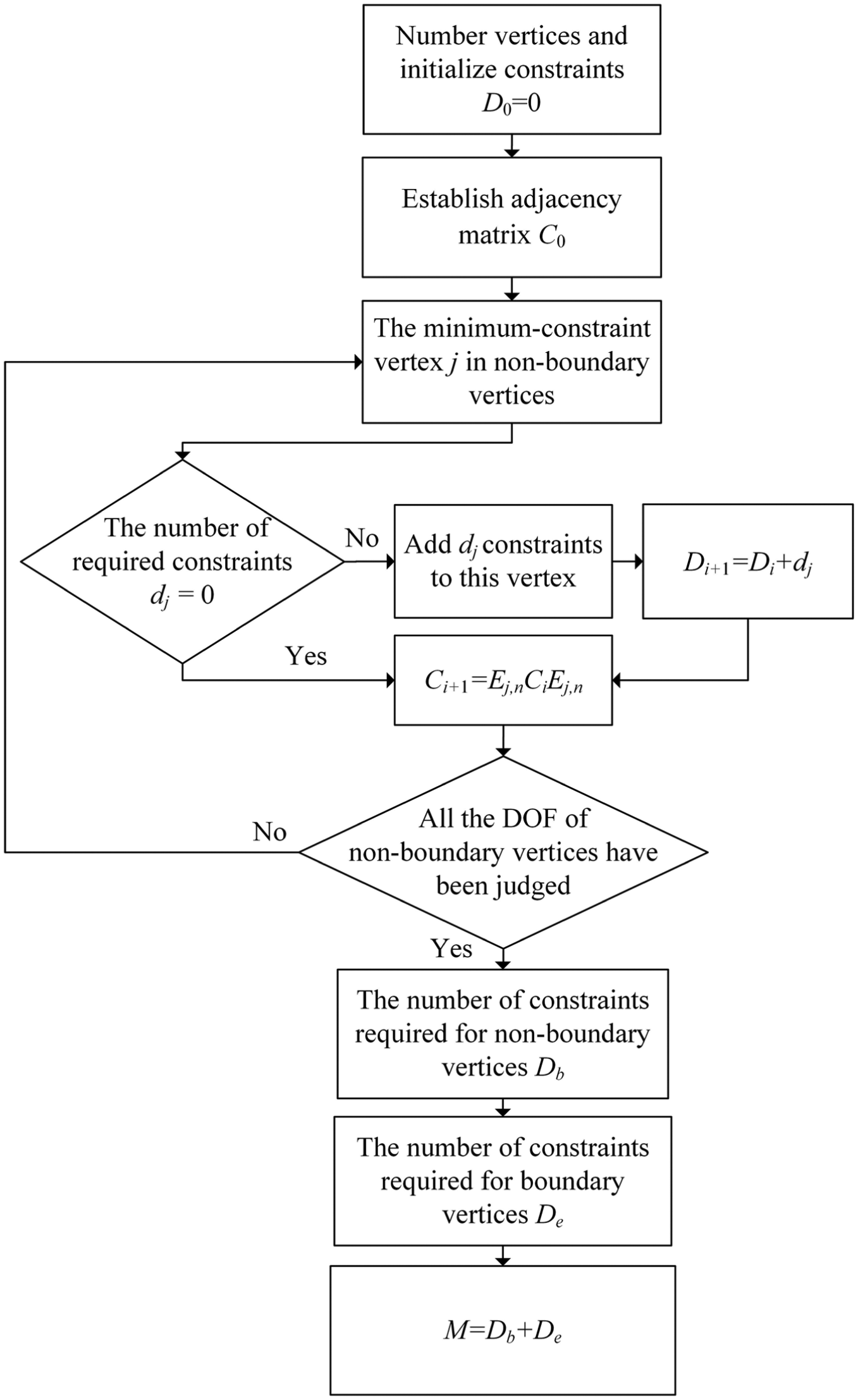
The analysis process of the DOF of multi-vertices.

The DOF of the pattern with multi-vertices, $M$ , is equal to the total number of constraints added when the motion of all vertices has been fully determined. That is, $M = D_{b} + D_{e}$ .

Redundant constraint judgment

The adjacency matrix method can determine the number of redundant constraints and the location of redundant constraints in the analysis process. Judging the redundant constraints by adjacency matrix method is introduced by taking Miura-ori pattern as an example. The empirical formula for calculating the DOF of rigid origami is

M = e - 3 b

(15)

where $e$ is the number of non-boundary edges in the rigid origami and $b$ is the number of non-boundary vertices.

The Miura-ori pattern shown in Figure 4 has 12 vertices and 31 edges except the boundary and boundary vertices. According to the empirical formula, the DOF of the pattern shown in Figure 4 is $- 5$ . In fact, the DOF of Miura-ori is 1. There are redundant constraints in the Miura-ori, and the redundant constraint is not considered when the empirical formula is used to calculate the DOF.

Figure 4.

Miura-ori.

Take the vertex with six creases in Figure 5 as an example to explain redundant constraints. Equation (4) shows that the DOF of the non-boundary vertex is equal to the number of edges minus 3, and that the DOF of this vertex is 3. When the rotation angles of the six creases are all uncertain, three constraints are required to completely determine the motion of the vertex. When the rotation angles of the creases $l_{1}$ , $l_{2}$ , and $l_{3}$ are all given values, though the rotation angles of the remaining three creases are not given, they are also the definite values. When the rotation angles of the creases $l_{1}$ , $l_{2}$ , $l_{3}$ , and $l_{4}$ are all given values, as the motion of the vertex with six creases can be determined by only three constraints, there is one redundant constraint at this vertex. When the rotation angles of the five creases are given, there are two redundant constraints. When the rotation angles of the six creases are all given, there are three redundant constraints. In the analysis of the DOF by the adjacency matrix method, the sum $\sum r_{i} (j)$ of the elements of each row represents the number of edges whose rotation angles are not given by the vertex corresponding to the row. By judging the situation of $\sum r_{i} (j) < 3$ in the analysis process, the redundant constraints of the rigid origami can be judged. When $\sum r_{i} (j) = 2$ , the number of redundant constraints of this vertex is one. When $\sum r_{i} (j) = 1$ , the number of redundant constraints of this vertex is two. When $\sum r_{i} (j) = 0$ , the number of redundant constraints of this vertex is three.

Figure 5.

The vertex with six creases.

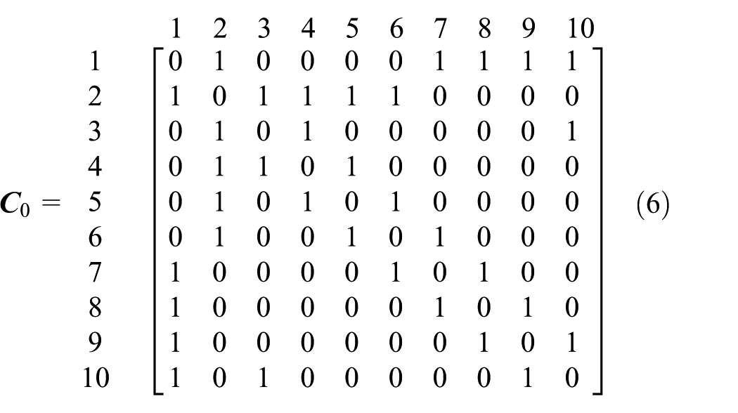
The analysis of redundant constraint of the Miura-ori shown in Figure 4 is now carried out. The adjacency matrix of the Miura-ori is

C_{0} = [\begin{matrix} 0 & 1 & 0 & 0 & 1 & 0 & 0 & 0 & 0 & 0 & 0 & 0 & 0 & 0 & 0 & 0 & 0 & 0 & 0 & 0 & 0 & 1 & 0 & 1 & 0 & 0 & 0 & 0 & 0 & 0 \\ 1 & 0 & 1 & 0 & 0 & 1 & 0 & 0 & 0 & 0 & 0 & 0 & 0 & 0 & 0 & 0 & 0 & 0 & 0 & 0 & 0 & 0 & 0 & 0 & 1 & 0 & 0 & 0 & 0 & 0 \\ 0 & 1 & 0 & 1 & 0 & 0 & 1 & 0 & 0 & 0 & 0 & 0 & 0 & 0 & 0 & 0 & 0 & 0 & 0 & 0 & 0 & 0 & 0 & 0 & 0 & 1 & 0 & 0 & 0 & 0 \\ 0 & 0 & 1 & 0 & 0 & 0 & 0 & 1 & 0 & 0 & 0 & 0 & 0 & 0 & 0 & 0 & 0 & 0 & 0 & 0 & 0 & 0 & 0 & 0 & 0 & 0 & 1 & 0 & 1 & 0 \\ 1 & 0 & 0 & 0 & 0 & 1 & 0 & 0 & 1 & 0 & 0 & 0 & 0 & 0 & 0 & 0 & 0 & 0 & 0 & 0 & 1 & 0 & 0 & 0 & 0 & 0 & 0 & 0 & 0 & 0 \\ 0 & 1 & 0 & 0 & 1 & 0 & 1 & 0 & 0 & 1 & 0 & 0 & 0 & 0 & 0 & 0 & 0 & 0 & 0 & 0 & 0 & 0 & 0 & 0 & 0 & 0 & 0 & 0 & 0 & 0 \\ 0 & 0 & 1 & 0 & 0 & 1 & 0 & 1 & 0 & 0 & 1 & 0 & 0 & 0 & 0 & 0 & 0 & 0 & 0 & 0 & 0 & 0 & 0 & 0 & 0 & 0 & 0 & 0 & 0 & 0 \\ 0 & 0 & 0 & 1 & 0 & 0 & 1 & 0 & 0 & 0 & 0 & 1 & 0 & 0 & 0 & 0 & 0 & 0 & 0 & 0 & 0 & 0 & 0 & 0 & 0 & 0 & 0 & 0 & 0 & 1 \\ 0 & 0 & 0 & 0 & 1 & 0 & 0 & 0 & 0 & 1 & 0 & 0 & 0 & 0 & 0 & 0 & 0 & 1 & 0 & 1 & 0 & 0 & 0 & 0 & 0 & 0 & 0 & 0 & 0 & 0 \\ 0 & 0 & 0 & 0 & 0 & 1 & 0 & 0 & 1 & 0 & 1 & 0 & 0 & 0 & 0 & 0 & 1 & 0 & 0 & 0 & 0 & 0 & 0 & 0 & 0 & 0 & 0 & 0 & 0 & 0 \\ 0 & 0 & 0 & 0 & 0 & 0 & 1 & 0 & 0 & 1 & 0 & 1 & 0 & 0 & 0 & 1 & 0 & 0 & 0 & 0 & 0 & 0 & 0 & 0 & 0 & 0 & 0 & 0 & 0 & 0 \\ 0 & 0 & 0 & 0 & 0 & 0 & 0 & 1 & 0 & 0 & 1 & 0 & 1 & 0 & 1 & 0 & 0 & 0 & 0 & 0 & 0 & 0 & 0 & 0 & 0 & 0 & 0 & 0 & 0 & 0 \\ 0 & 0 & 0 & 0 & 0 & 0 & 0 & 0 & 0 & 0 & 0 & 1 & 0 & 1 & 0 & 0 & 0 & 0 & 0 & 0 & 0 & 0 & 0 & 0 & 0 & 0 & 0 & 0 & 0 & 1 \\ 0 & 0 & 0 & 0 & 0 & 0 & 0 & 0 & 0 & 0 & 0 & 0 & 1 & 0 & 1 & 0 & 0 & 0 & 0 & 0 & 0 & 0 & 0 & 0 & 0 & 0 & 0 & 0 & 0 & 0 \\ 0 & 0 & 0 & 0 & 0 & 0 & 0 & 0 & 0 & 0 & 0 & 1 & 0 & 1 & 0 & 1 & 0 & 0 & 0 & 0 & 0 & 0 & 0 & 0 & 0 & 0 & 0 & 0 & 0 & 0 \\ 0 & 0 & 0 & 0 & 0 & 0 & 0 & 0 & 0 & 0 & 1 & 0 & 0 & 0 & 1 & 0 & 1 & 0 & 0 & 0 & 0 & 0 & 0 & 0 & 0 & 0 & 0 & 0 & 0 & 0 \\ 0 & 0 & 0 & 0 & 0 & 0 & 0 & 0 & 0 & 1 & 0 & 0 & 0 & 0 & 0 & 1 & 0 & 1 & 0 & 0 & 0 & 0 & 0 & 0 & 0 & 0 & 0 & 0 & 0 & 0 \\ 0 & 0 & 0 & 0 & 0 & 0 & 0 & 0 & 1 & 0 & 0 & 0 & 0 & 0 & 0 & 0 & 1 & 0 & 1 & 0 & 0 & 0 & 0 & 0 & 0 & 0 & 0 & 0 & 0 & 0 \\ 0 & 0 & 0 & 0 & 0 & 0 & 0 & 0 & 0 & 0 & 0 & 0 & 0 & 0 & 0 & 0 & 0 & 1 & 0 & 1 & 0 & 0 & 0 & 0 & 0 & 0 & 0 & 0 & 0 & 0 \\ 0 & 0 & 0 & 0 & 0 & 0 & 0 & 0 & 1 & 0 & 0 & 0 & 0 & 0 & 0 & 0 & 0 & 0 & 1 & 0 & 1 & 0 & 0 & 0 & 0 & 0 & 0 & 0 & 0 & 0 \\ 0 & 0 & 0 & 0 & 1 & 0 & 0 & 0 & 0 & 0 & 0 & 0 & 0 & 0 & 0 & 0 & 0 & 0 & 0 & 1 & 0 & 1 & 0 & 0 & 0 & 0 & 0 & 0 & 0 & 0 \\ 1 & 0 & 0 & 0 & 0 & 0 & 0 & 0 & 0 & 0 & 0 & 0 & 0 & 0 & 0 & 0 & 0 & 0 & 0 & 0 & 1 & 0 & 1 & 0 & 0 & 0 & 0 & 0 & 0 & 0 \\ 0 & 0 & 0 & 0 & 0 & 0 & 0 & 0 & 0 & 0 & 0 & 0 & 0 & 0 & 0 & 0 & 0 & 0 & 0 & 0 & 0 & 1 & 0 & 1 & 0 & 0 & 0 & 0 & 0 & 0 \\ 1 & 0 & 0 & 0 & 0 & 0 & 0 & 0 & 0 & 0 & 0 & 0 & 0 & 0 & 0 & 0 & 0 & 0 & 0 & 0 & 0 & 0 & 1 & 0 & 1 & 0 & 0 & 0 & 0 & 0 \\ 0 & 1 & 0 & 0 & 0 & 0 & 0 & 0 & 0 & 0 & 0 & 0 & 0 & 0 & 0 & 0 & 0 & 0 & 0 & 0 & 0 & 0 & 0 & 1 & 0 & 1 & 0 & 0 & 0 & 0 \\ 0 & 0 & 1 & 0 & 0 & 0 & 0 & 0 & 0 & 0 & 0 & 0 & 0 & 0 & 0 & 0 & 0 & 0 & 0 & 0 & 0 & 0 & 0 & 0 & 1 & 0 & 1 & 0 & 0 & 0 \\ 0 & 0 & 0 & 1 & 0 & 0 & 0 & 0 & 0 & 0 & 0 & 0 & 0 & 0 & 0 & 0 & 0 & 0 & 0 & 0 & 0 & 0 & 0 & 0 & 0 & 1 & 0 & 1 & 0 & 0 \\ 0 & 0 & 0 & 0 & 0 & 0 & 0 & 0 & 0 & 0 & 0 & 0 & 0 & 0 & 0 & 0 & 0 & 0 & 0 & 0 & 0 & 0 & 0 & 0 & 0 & 0 & 1 & 0 & 1 & 0 \\ 0 & 0 & 0 & 1 & 0 & 0 & 0 & 0 & 0 & 0 & 0 & 0 & 0 & 0 & 0 & 0 & 0 & 0 & 0 & 0 & 0 & 0 & 0 & 0 & 0 & 0 & 0 & 1 & 0 & 1 \\ 0 & 0 & 0 & 0 & 0 & 0 & 0 & 1 & 0 & 0 & 0 & 0 & 1 & 0 & 0 & 0 & 0 & 0 & 0 & 0 & 0 & 0 & 0 & 0 & 0 & 0 & 0 & 0 & 1 & 0 \end{matrix}]

(16)

According to the analysis procedure shown in Figure 3, the minimum-constraint vertex is determined and the elimination transformation is performed. There are a variety of elimination paths in this pattern, and the position of redundant constraints is different in different elimination paths, but the total number of redundant constraints is the same. Only one elimination path is listed here, $1 \to 2 \to 3 \to 4 \to 5 \to 6 \to 7 \to 8 \to 9 \to 10 \to 11 \to 12$ . The elimination transformation is performed only among the non-boundary vertices. The DOF of the boundary vertices is calculated according to equation (14) after the elimination transformation. One constraint is added to vertex 1, and then the elimination transformation is performed. After the fifth elimination transformation, the matrix $C_{5}$ is

C_{5} = [\begin{matrix} 0 & 0 & 0 & 0 & 0 & 0 & 0 & 0 & 0 & 0 & 0 & 0 & 0 & 0 & 0 & 0 & 0 & 0 & 0 & 0 & 0 & 0 & 0 & 0 & 0 & 0 & 0 & 0 & 0 & 0 \\ 0 & 0 & 0 & 0 & 0 & 0 & 0 & 0 & 0 & 0 & 0 & 0 & 0 & 0 & 0 & 0 & 0 & 0 & 0 & 0 & 0 & 0 & 0 & 0 & 0 & 0 & 0 & 0 & 0 & 0 \\ 0 & 0 & 0 & 0 & 0 & 0 & 0 & 0 & 0 & 0 & 0 & 0 & 0 & 0 & 0 & 0 & 0 & 0 & 0 & 0 & 0 & 0 & 0 & 0 & 0 & 0 & 0 & 0 & 0 & 0 \\ 0 & 0 & 0 & 0 & 0 & 0 & 0 & 0 & 0 & 0 & 0 & 0 & 0 & 0 & 0 & 0 & 0 & 0 & 0 & 0 & 0 & 0 & 0 & 0 & 0 & 0 & 0 & 0 & 0 & 0 \\ 0 & 0 & 0 & 0 & 0 & 0 & 0 & 0 & 0 & 0 & 0 & 0 & 0 & 0 & 0 & 0 & 0 & 0 & 0 & 0 & 0 & 0 & 0 & 0 & 0 & 0 & 0 & 0 & 0 & 0 \\ 0 & 0 & 0 & 0 & 0 & 0 & 1 & 0 & 0 & 1 & 0 & 0 & 0 & 0 & 0 & 0 & 0 & 0 & 0 & 0 & 0 & 0 & 0 & 0 & 0 & 0 & 0 & 0 & 0 & 0 \\ 0 & 0 & 0 & 0 & 0 & 1 & 0 & 1 & 0 & 0 & 1 & 0 & 0 & 0 & 0 & 0 & 0 & 0 & 0 & 0 & 0 & 0 & 0 & 0 & 0 & 0 & 0 & 0 & 0 & 0 \\ 0 & 0 & 0 & 0 & 0 & 0 & 1 & 0 & 0 & 0 & 0 & 1 & 0 & 0 & 0 & 0 & 0 & 0 & 0 & 0 & 0 & 0 & 0 & 0 & 0 & 0 & 0 & 0 & 0 & 1 \\ 0 & 0 & 0 & 0 & 0 & 0 & 0 & 0 & 0 & 1 & 0 & 0 & 0 & 0 & 0 & 0 & 0 & 1 & 0 & 1 & 0 & 0 & 0 & 0 & 0 & 0 & 0 & 0 & 0 & 0 \\ 0 & 0 & 0 & 0 & 0 & 1 & 0 & 0 & 1 & 0 & 1 & 0 & 0 & 0 & 0 & 0 & 1 & 0 & 0 & 0 & 0 & 0 & 0 & 0 & 0 & 0 & 0 & 0 & 0 & 0 \\ 0 & 0 & 0 & 0 & 0 & 0 & 1 & 0 & 0 & 1 & 0 & 1 & 0 & 0 & 0 & 1 & 0 & 0 & 0 & 0 & 0 & 0 & 0 & 0 & 0 & 0 & 0 & 0 & 0 & 0 \\ 0 & 0 & 0 & 0 & 0 & 0 & 0 & 1 & 0 & 0 & 1 & 0 & 1 & 0 & 1 & 0 & 0 & 0 & 0 & 0 & 0 & 0 & 0 & 0 & 0 & 0 & 0 & 0 & 0 & 0 \\ 0 & 0 & 0 & 0 & 0 & 0 & 0 & 0 & 0 & 0 & 0 & 1 & 0 & 1 & 0 & 0 & 0 & 0 & 0 & 0 & 0 & 0 & 0 & 0 & 0 & 0 & 0 & 0 & 0 & 1 \\ 0 & 0 & 0 & 0 & 0 & 0 & 0 & 0 & 0 & 0 & 0 & 0 & 1 & 0 & 1 & 0 & 0 & 0 & 0 & 0 & 0 & 0 & 0 & 0 & 0 & 0 & 0 & 0 & 0 & 0 \\ 0 & 0 & 0 & 0 & 0 & 0 & 0 & 0 & 0 & 0 & 0 & 1 & 0 & 1 & 0 & 1 & 0 & 0 & 0 & 0 & 0 & 0 & 0 & 0 & 0 & 0 & 0 & 0 & 0 & 0 \\ 0 & 0 & 0 & 0 & 0 & 0 & 0 & 0 & 0 & 0 & 1 & 0 & 0 & 0 & 1 & 0 & 1 & 0 & 0 & 0 & 0 & 0 & 0 & 0 & 0 & 0 & 0 & 0 & 0 & 0 \\ 0 & 0 & 0 & 0 & 0 & 0 & 0 & 0 & 0 & 1 & 0 & 0 & 0 & 0 & 0 & 1 & 0 & 1 & 0 & 0 & 0 & 0 & 0 & 0 & 0 & 0 & 0 & 0 & 0 & 0 \\ 0 & 0 & 0 & 0 & 0 & 0 & 0 & 0 & 1 & 0 & 0 & 0 & 0 & 0 & 0 & 0 & 1 & 0 & 1 & 0 & 0 & 0 & 0 & 0 & 0 & 0 & 0 & 0 & 0 & 0 \\ 0 & 0 & 0 & 0 & 0 & 0 & 0 & 0 & 0 & 0 & 0 & 0 & 0 & 0 & 0 & 0 & 0 & 1 & 0 & 1 & 0 & 0 & 0 & 0 & 0 & 0 & 0 & 0 & 0 & 0 \\ 0 & 0 & 0 & 0 & 0 & 0 & 0 & 0 & 1 & 0 & 0 & 0 & 0 & 0 & 0 & 0 & 0 & 0 & 1 & 0 & 1 & 0 & 0 & 0 & 0 & 0 & 0 & 0 & 0 & 0 \\ 0 & 0 & 0 & 0 & 0 & 0 & 0 & 0 & 0 & 0 & 0 & 0 & 0 & 0 & 0 & 0 & 0 & 0 & 0 & 1 & 0 & 1 & 0 & 0 & 0 & 0 & 0 & 0 & 0 & 0 \\ 0 & 0 & 0 & 0 & 0 & 0 & 0 & 0 & 0 & 0 & 0 & 0 & 0 & 0 & 0 & 0 & 0 & 0 & 0 & 0 & 1 & 0 & 1 & 0 & 0 & 0 & 0 & 0 & 0 & 0 \\ 0 & 0 & 0 & 0 & 0 & 0 & 0 & 0 & 0 & 0 & 0 & 0 & 0 & 0 & 0 & 0 & 0 & 0 & 0 & 0 & 0 & 1 & 0 & 1 & 0 & 0 & 0 & 0 & 0 & 0 \\ 0 & 0 & 0 & 0 & 0 & 0 & 0 & 0 & 0 & 0 & 0 & 0 & 0 & 0 & 0 & 0 & 0 & 0 & 0 & 0 & 0 & 0 & 1 & 0 & 1 & 0 & 0 & 0 & 0 & 0 \\ 0 & 0 & 0 & 0 & 0 & 0 & 0 & 0 & 0 & 0 & 0 & 0 & 0 & 0 & 0 & 0 & 0 & 0 & 0 & 0 & 0 & 0 & 0 & 1 & 0 & 1 & 0 & 0 & 0 & 0 \\ 0 & 0 & 0 & 0 & 0 & 0 & 0 & 0 & 0 & 0 & 0 & 0 & 0 & 0 & 0 & 0 & 0 & 0 & 0 & 0 & 0 & 0 & 0 & 0 & 1 & 0 & 1 & 0 & 0 & 0 \\ 0 & 0 & 0 & 0 & 0 & 0 & 0 & 0 & 0 & 0 & 0 & 0 & 0 & 0 & 0 & 0 & 0 & 0 & 0 & 0 & 0 & 0 & 0 & 0 & 0 & 1 & 0 & 1 & 0 & 0 \\ 0 & 0 & 0 & 0 & 0 & 0 & 0 & 0 & 0 & 0 & 0 & 0 & 0 & 0 & 0 & 0 & 0 & 0 & 0 & 0 & 0 & 0 & 0 & 0 & 0 & 0 & 1 & 0 & 1 & 0 \\ 0 & 0 & 0 & 0 & 0 & 0 & 0 & 0 & 0 & 0 & 0 & 0 & 0 & 0 & 0 & 0 & 0 & 0 & 0 & 0 & 0 & 0 & 0 & 0 & 0 & 0 & 0 & 1 & 0 & 1 \\ 0 & 0 & 0 & 0 & 0 & 0 & 0 & 1 & 0 & 0 & 0 & 0 & 1 & 0 & 0 & 0 & 0 & 0 & 0 & 0 & 0 & 0 & 0 & 0 & 0 & 0 & 0 & 0 & 1 & 0 \end{matrix}]

(17)

The sixth row $r_{5} (6)$ of the matrix $C_{5}$ obtained by five elimination transformations, is $[\begin{matrix} 0 & 0 & 0 & 0 & 0 & 0 & 1 & 0 & 0 & 1 & 0 & 0 & 0 & 0 & 0 & 0 & 0 & 0 & 0 & 0 & 0 & 0 & 0 & 0 & 0 & 0 & 0 & 0 & 0 & 0 \end{matrix}]$ . The sum of the elements of the row $\sum r_{5} (6)$ is 2, less than 3, and there is a redundant constraint at the vertex 6 when we analyze along this elimination path. Continue the elimination transformation (no more matrices are listed here), and the seventh row $r_{6} (7)$ of the matrix $C_{6}$ obtained by six elimination transformations is $[\begin{matrix} 0 & 0 & 0 & 0 & 0 & 0 & 0 & 1 & 0 & 0 & 1 & 0 & 0 & 0 & 0 & 0 & 0 & 0 & 0 & 0 & 0 & 0 & 0 & 0 & 0 & 0 & 0 & 0 & 0 & 0 \end{matrix}]$

The eighth row $r_{7} (8)$ of the matrix $C_{7}$ obtained by seven elimination transformations is $[\begin{matrix} 0 & 0 & 0 & 0 & 0 & 0 & 0 & 0 & 0 & 0 & 0 & 1 & 0 & 0 & 0 & 0 & 0 & 0 & 0 & 0 & 0 & 0 & 0 & 0 & 0 & 0 & 0 & 0 & 0 & 1 \end{matrix}]$ .

The 10th row $r_{9} (10)$ of the matrix $C_{9}$ obtained by nine elimination transformations is $[\begin{matrix} 0 & 0 & 0 & 0 & 0 & 0 & 0 & 0 & 0 & 0 & 1 & 0 & 0 & 0 & 0 & 0 & 1 & 0 & 0 & 0 & 0 & 0 & 0 & 0 & 0 & 0 & 0 & 0 & 0 & 0 \end{matrix}]$ .

The 11th row $r_{10} (11)$ of the matrix $C_{10}$ obtained by 10 elimination transformations is $[\begin{matrix} 0 & 0 & 0 & 0 & 0 & 0 & 0 & 0 & 0 & 0 & 0 & 1 & 0 & 0 & 0 & 1 & 0 & 0 & 0 & 0 & 0 & 0 & 0 & 0 & 0 & 0 & 0 & 0 & 0 & 0 \end{matrix}]$ .

The 12th row $r_{11} (12)$ of the matrix $C_{11}$ obtained by 11 elimination transformations is $[\begin{matrix} 0 & 0 & 0 & 0 & 0 & 0 & 0 & 0 & 0 & 0 & 0 & 0 & 1 & 0 & 1 & 0 & 0 & 0 & 0 & 0 & 0 & 0 & 0 & 0 & 0 & 0 & 0 & 0 & 0 & 0 \end{matrix}]$ .

The sum of the elements in each rows is 2. That is, there is one redundant constraint at each vertex 6, 7, 8, 10, 11, and 12. The total number of redundant constraints is six. According to the empirical formula, the DOF of this pattern is $- 5$ . That is, the DOF determined by empirical formula plus the number of redundant constraints equals the actual DOF of the pattern.

Exceptional case

Cross-crease vertex

The distribution of the four creases in the cross-crease vertex³⁴ is shown in Figure 6(a). The two opposite creases are collinear, that is, the angles between the creases satisfy the condition $α_{12} = α_{34} = α$ , and $α_{23} = α_{41} = π - α$ . The cross-crease vertex has two states of motion, one is shown in Figure 6(b), $θ_{2} = θ_{4} = 0$ , $θ_{1} = θ_{3}$ , the other is shown in Figure 6(c), $θ_{1} = θ_{3} = 0$ , $θ_{2} = θ_{4}$ . When a crease has a non-zero rotation angle $θ$ , the motion of its adjacent crease is suppressed.

Figure 6.

The cross-crease vertex and its fold states: (a) the cross-crease vertex, (b) one fold state, and (c) the other fold state.

For cross-crease vertex, when the rotation angle of a crease is not 0, it can be determined that the rotation angle of the adjacent crease is 0, but when the rotation angle of the crease is 0, the rotation angle of the adjacent crease cannot be determined. According to the kinematic characteristics of the cross creases, the origami pattern shown in Figure 7(a) has two motion states, as shown in Figure 7(b) and (c). As shown in Figure 7(b), the intersection of creases 1, 2, 3, and 4 is cross-crease vertex. The rotation angle of crease 1 is non-zero angle $θ_{1}$ , then $θ_{2} = θ_{4} = 0$ and $θ_{3} = θ_{1}$ . The intersection of creases 3, 10, 11, and 12 is cross-crease vertex. The rotation angle of crease 3 is non-zero angle $θ_{3}$ , then $θ_{10} = θ_{12} = 0$ and $θ_{11} = θ_{3} = θ_{1}$ . According to equation (4), the non-boundary vertex with four creases has a single DOF, that is, the rotation angle of the other creases is determined as long as the rotation angle of any crease is determined. The intersection of creases 2, 5, 6, and 7 is also cross-crease vertex. Now the rotation angle $θ_{2}$ is determined, $θ_{2} = 0$ . By the above analysis, the data of $θ_{5}$ , $θ_{6}$ , and $θ_{7}$ should also be determined. But in fact, when $θ_{2}$ is 0, it can only determine the rotation angle of the opposite crease, $θ_{6} = 0$ , and the rotation angle $θ_{5}$ and $θ_{7}$ of its adjacent creases cannot be determined.

Figure 7.

Origami pattern with many cross-crease vertices and its fold states: (a) origami pattern with many cross-crease vertices, (b) one fold state, and (c) the other fold state.

The above properties of cross-crease vertex result in possible errors when judging DOF using the adjacency matrix method. In order to avoid errors, the creases can be classified and simplified. According to the kinematic properties of cross-crease vertex, the vertex has only two motion states, and only one state can be represented at one time. When one crease of a cross-crease vertex has a non-zero rotation angle, the rotation angle of its adjacent crease must be zero. When the rotation angle of one crease is zero, the rotation angle of its opposite crease must be zero. If we classify and simplify the creases of cross-crease vertices, the corresponding creases can be ignored according to the motion trend at the vertex. The pattern shown in Figure 7(a) can be classified and simplified as pattern shown in Figure 8(a) and (b). If the crease 1 in Figure 7(a) has non-zero rotation angle, then the pattern in Figure 7(a) is equivalent to the pattern in Figure 8(a). If the crease 4 in Figure 7(a) has non-zero rotation angle, then the pattern in Figure 7(a) is equivalent to the pattern in Figure 8(b). The adjacency matrix is established by the simplified pattern shown in Figure 8, to analyze the DOF of multi-vertices, then the misjudgment caused by cross-crease vertex can be avoided.

Figure 8.

Simplified pattern: (a) the transverse creases are ignored and (b) the longitudinal creases are ignored.

Ring pattern

As for the ring pattern shown in Figure 9(a), all the vertices of the inner ring and the outer ring are the boundary vertices, and there is error when calculating the DOF by directly using the adjacency matrix method. The four creases of the pattern will intersect at the same point (as shown in Figure 9(b)). The patterns shown in Figure 9(a) and (b) have the same motion characteristics due to the same direction and position of the creases. The folding states of the two patterns are shown in Figure 10. For the ring pattern with creases intersecting at the same point, the creases can be extended, then the pattern is equivalent to a pattern with single vertex pattern. The DOF of this pattern can be obtained by analyzing the DOF of the equivalent pattern using the adjacency matrix method. The DOF of the pattern shown in Figure 9(a) is 1.

Figure 9.

Ring pattern with four creases and the pattern with single vertex: (a) ring pattern with four creases and (b) the pattern with single vertex.

Figure 10.

Folding states of the ring pattern and pattern with single vertex: (a) folding state of the ring pattern and (b) folding state of the pattern with single vertex.

As shown in Figure 11(a), the creases of some ring patterns do not intersect at the same point. In this case, the ring pattern cannot be simply equivalent to the pattern with a single vertex. The DOF can be calculated from the dimension of the null space of the Jacobian matrix.²⁶ The DOF of this pattern is 1, and the calculation process is shown in Appendix 1.

Figure 11.

Ring pattern with six creases and its folding state: (a) ring pattern with six creases and (b) folding state of the ring pattern.

For the pattern consisting of multiple ring patterns (shown in Figure 12(a)), calculating the dimension of the null space of the Jacobian matrix is complex. The method combining the null space of the Jacobian matrix and the adjacency matrix can be used.

Figure 12.

The whole pattern with multiple ring patterns and its folding state: (a) the whole pattern and (b) folding state of the whole pattern.

The pattern shown in Figure 12(a) is composed of four patterns shown in Figure 11(a). To analyze the DOF of this pattern, simplify the pattern shown in Figure 11(a) first, and then the whole configuration can be simplified. The pattern shown in Figure 11(a) can be replaced by an imaginary simplified pattern with single vertex shown in Figure 13(a). The number of creases which intersect at the same point in the simplified pattern is the same as that in the ring pattern. The simplified pattern is only an ideal pattern without real existence, only for the convenience of calculating the DOF of the pattern shown in Figure 12(a). The DOF of the simplified pattern is different from that of the ordinary single vertex with six creases, but the same as that of the pattern shown in Figure 11(a), and both of which are 1. The method to calculate the DOF of the simplified pattern becomes

M = m - 5

(18)

Figure 13.

The simplified pattern: (a) the simplified pattern of ring pattern with six creases and (b) the simplified pattern of the whole pattern.

It is shown that the number of constraints required to determine the motion of vertex 1 is equal to the number of “1s” in the row element corresponding to the vertex 1 in the adjacency matrix minus 5. For example, the first row element corresponding to the vertex 1 of the initial adjacency matrix of the pattern shown in Figure 13(a) is $r_{1} = [\begin{matrix} 0 & 1 & 1 & 1 & 1 & 1 & 1 \end{matrix}]$ . Vertex 1 is the imaginary intersection point, and its DOF is calculated in accordance with equation (18). The number of elements “1” in the first row is 6, and the DOF of this vertex is 1.

The ring patterns shown in Figure 12(a) are all simplified as the pattern shown in Figure 13(a), and the whole pattern after simplification is shown in Figure 13(b). In Figure 13(b), vertices 1, 2, 5, and 6 are imaginary intersections, whose DOFs are calculated in accordance with equation (18). Vertices 3 and 4 are the non-boundary vertices, whose DOFs are calculated according to equation (4). The rest of the vertices are the original boundary vertices, whose DOFs are calculated in accordance with equation (5).

The calculation of the DOF of the pattern shown in Figure 13(b) is as follows, and the initial adjacency matrix is established as

C_{0} = [\begin{matrix} 0 & 0 & 1 & 1 & 0 & 0 & 1 & 1 & 0 & 0 & 0 & 0 & 0 & 0 & 0 & 0 & 0 & 0 & 1 & 1 \\ 0 & 0 & 1 & 0 & 0 & 0 & 0 & 1 & 1 & 1 & 1 & 1 & 0 & 0 & 0 & 0 & 0 & 0 & 0 & 0 \\ 1 & 1 & 0 & 1 & 0 & 1 & 0 & 1 & 0 & 0 & 0 & 1 & 0 & 0 & 0 & 0 & 0 & 0 & 0 & 0 \\ 1 & 0 & 1 & 0 & 1 & 1 & 0 & 0 & 0 & 0 & 0 & 0 & 0 & 0 & 1 & 0 & 0 & 0 & 1 & 0 \\ 0 & 0 & 0 & 1 & 0 & 0 & 0 & 0 & 0 & 0 & 0 & 0 & 0 & 0 & 1 & 1 & 1 & 1 & 1 & 0 \\ 0 & 0 & 1 & 1 & 0 & 0 & 0 & 0 & 0 & 0 & 0 & 1 & 1 & 1 & 1 & 0 & 0 & 0 & 0 & 0 \\ 1 & 0 & 0 & 0 & 0 & 0 & 0 & 1 & 0 & 0 & 0 & 0 & 0 & 0 & 0 & 0 & 0 & 0 & 0 & 1 \\ 1 & 1 & 1 & 0 & 0 & 0 & 1 & 0 & 1 & 0 & 0 & 0 & 0 & 0 & 0 & 0 & 0 & 0 & 0 & 0 \\ 0 & 1 & 0 & 0 & 0 & 0 & 0 & 1 & 0 & 1 & 0 & 0 & 0 & 0 & 0 & 0 & 0 & 0 & 0 & 0 \\ 0 & 1 & 0 & 0 & 0 & 0 & 0 & 0 & 1 & 0 & 1 & 0 & 0 & 0 & 0 & 0 & 0 & 0 & 0 & 0 \\ 0 & 1 & 0 & 0 & 0 & 0 & 0 & 0 & 0 & 1 & 0 & 1 & 0 & 0 & 0 & 0 & 0 & 0 & 0 & 0 \\ 0 & 1 & 1 & 0 & 0 & 1 & 0 & 0 & 0 & 0 & 1 & 0 & 1 & 0 & 0 & 0 & 0 & 0 & 0 & 0 \\ 0 & 0 & 0 & 0 & 0 & 1 & 0 & 0 & 0 & 0 & 0 & 1 & 0 & 1 & 0 & 0 & 0 & 0 & 0 & 0 \\ 0 & 0 & 0 & 0 & 0 & 1 & 0 & 0 & 0 & 0 & 0 & 0 & 1 & 0 & 1 & 0 & 0 & 0 & 0 & 0 \\ 0 & 0 & 0 & 1 & 1 & 1 & 0 & 0 & 0 & 0 & 0 & 0 & 0 & 1 & 0 & 1 & 0 & 0 & 0 & 0 \\ 0 & 0 & 0 & 0 & 1 & 0 & 0 & 0 & 0 & 0 & 0 & 0 & 0 & 0 & 1 & 0 & 1 & 0 & 0 & 0 \\ 0 & 0 & 0 & 0 & 1 & 0 & 0 & 0 & 0 & 0 & 0 & 0 & 0 & 0 & 0 & 1 & 0 & 1 & 0 & 0 \\ 0 & 0 & 0 & 0 & 1 & 0 & 0 & 0 & 0 & 0 & 0 & 0 & 0 & 0 & 0 & 0 & 1 & 0 & 1 & 0 \\ 1 & 0 & 0 & 1 & 1 & 0 & 0 & 0 & 0 & 0 & 0 & 0 & 0 & 0 & 0 & 0 & 0 & 1 & 0 & 1 \\ 1 & 0 & 0 & 0 & 0 & 0 & 1 & 0 & 0 & 0 & 0 & 0 & 0 & 0 & 0 & 0 & 0 & 0 & 1 & 0 \end{matrix}]

(19)

According to the adjacency matrix method to judge DOF, first, the minimum-constraint vertex in the non-boundary vertices are determined. According to equation (18), the number of required constraints of vertices 1, 2, 5, and 6 are all 1. On the basis of equation (4), the number of required constraints of vertices 3 and 4 is 3. Then any vertices among 1, 2, 5, and 6 can be chosen as the minimum-constraint vertex, when doing the first elimination transformation. According to the principle of selecting the minimum-constraint to eliminate, the elimination path $1 \to 2 \to 3 \to 6 \to 4 \to 5$ is chosen to analyze the DOF. Note that the difference between the imaginary vertex and the true non-boundary vertex in determining the required constraint. According to the above elimination path, one constraint is provided for vertex 1, one constraint for vertex 2, and one constraint for vertex 3. The sixth row $r_{3} (6)$ of the matrix $C_{3}$ obtained by three elimination transformations is

r_{3} (6) = [\begin{matrix} 0 & 0 & 0 & 1 & 0 & 0 & 0 & 0 & 0 & 0 & 0 & 1 & 1 & 1 & 1 & 0 & 0 & 0 & 0 & 0 \end{matrix}]

There are 5 “1s” in this row. According to equation (18), the number of required constraints is 0, that is, there is no need to provide constraints, and the elimination transformation can be carried out.

The fifth row $r_{5} (5)$ of the matrix $C_{5}$ obtained by five elimination transformations is

r_{5} (5) = [\begin{matrix} 0 & 0 & 0 & 0 & 0 & 0 & 0 & 0 & 0 & 0 & 0 & 0 & 0 & 0 & 1 & 1 & 1 & 1 & 1 & 0 \end{matrix}]

Like vertex 6, there is no need for constraints at this vertex. When the motion of the non-boundary vertices is determined, the constraints required by the boundary vertices are calculated according to equation (14). The number of constraints required for the boundary vertices of this pattern is 0. After three constraints are added, the motion of the whole pattern is determined, that is DOF of this pattern is 3.

For other origami patterns like the pattern shown in Figure 12(a), which consists of a number of ring patterns, the DOF can be determined according to the above method. First, the number of constraints required for a single ring pattern is determined. For the ring pattern with creases that intersect at one point, after extending the creases, the pattern is considered as a pattern with single vertex. When the creases do not intersect at the same point, use the method of the Jacobian matrix²⁶ to calculate DOF. Then each ring pattern can be simplified to an imaginary pattern with single vertex. The number of creases in the simplified single vertex pattern is the same as that in the ring pattern, ignoring boundaries. Finally, the DOF of the whole pattern can be judged by the adjacency matrix method. Note that the method to calculate the number of constraints required for virtual vertices is different from that of general vertices.

Example analysis

Waterbomb

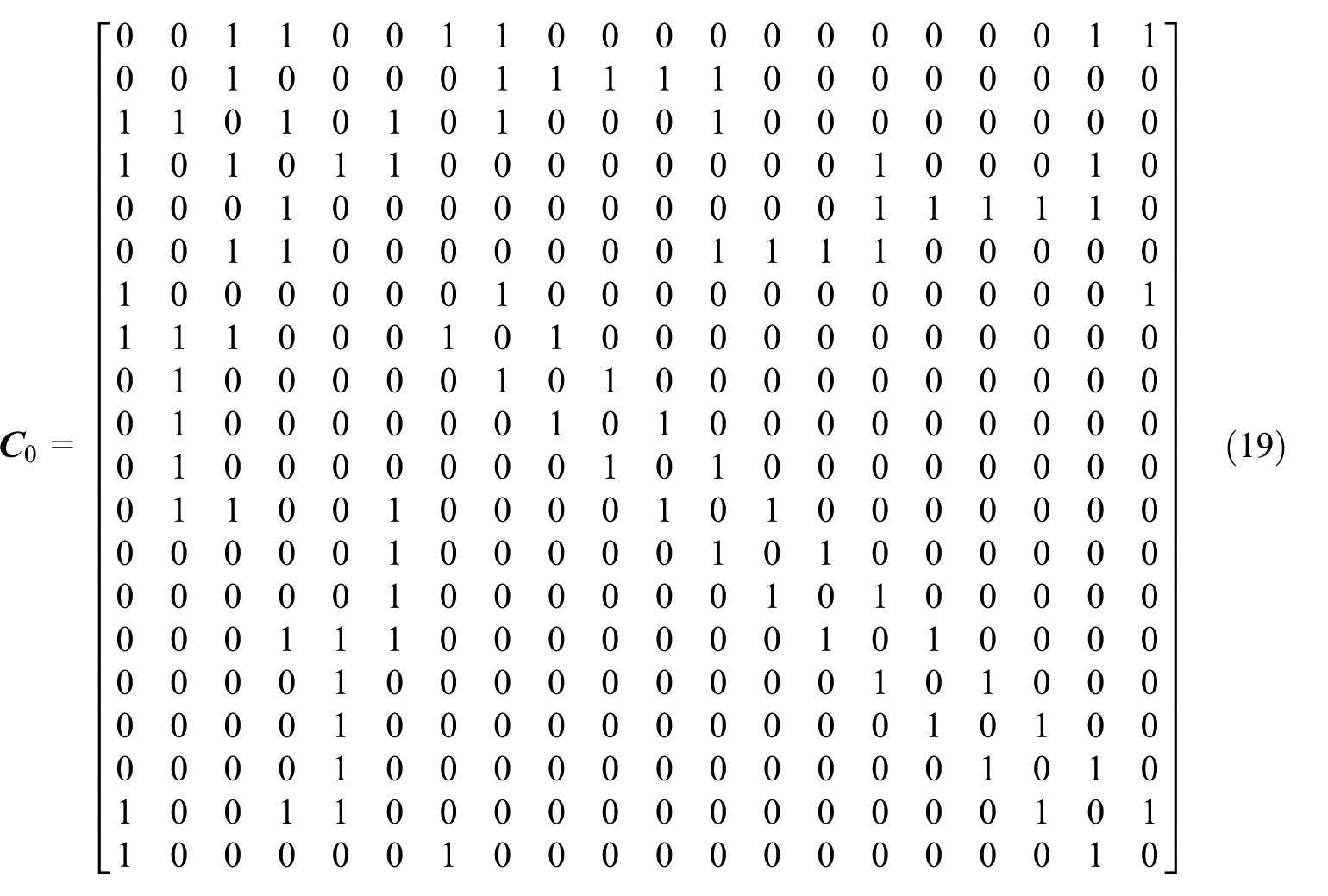
The DOF of the waterbomb^35,36 shown in Figure 14 is analyzed by the adjacency matrix method. First, the adjacency matrix is established as follows

C_{0} = [\begin{matrix} \begin{matrix} 0 & 0 & 0 & 1 & 1 & 0 & 0 & 0 & 0 & 0 & 0 & 0 & 0 & 0 & 0 & 0 \\ 0 & 0 & 0 & 0 & 1 & 1 & 1 & 0 & 0 & 0 & 0 & 0 & 0 & 0 & 0 & 0 \\ 0 & 0 & 0 & 0 & 0 & 0 & 1 & 1 & 1 & 0 & 0 & 0 & 0 & 0 & 0 & 0 \\ 1 & 0 & 0 & 0 & 1 & 0 & 0 & 0 & 0 & 1 & 0 & 0 & 0 & 0 & 0 & 0 \\ 1 & 1 & 0 & 1 & 0 & 1 & 0 & 0 & 0 & 1 & 0 & 0 & 0 & 0 & 0 & 0 \\ 0 & 1 & 0 & 0 & 1 & 0 & 1 & 0 & 0 & 1 & 1 & 0 & 0 & 0 & 0 & 0 \\ 0 & 1 & 1 & 0 & 0 & 1 & 0 & 1 & 0 & 0 & 1 & 0 & 0 & 0 & 0 & 0 \\ 0 & 0 & 1 & 0 & 0 & 0 & 1 & 0 & 1 & 0 & 1 & 1 & 0 & 0 & 1 & 0 \\ 0 & 0 & 1 & 0 & 0 & 0 & 0 & 1 & 0 & 0 & 0 & 1 & 0 & 0 & 0 & 0 \\ 0 & 0 & 0 & 1 & 1 & 1 & 0 & 0 & 0 & 0 & 0 & 0 & 0 & 0 & 0 & 0 \\ 0 & 0 & 0 & 0 & 0 & 1 & 1 & 1 & 0 & 0 & 0 & 0 & 0 & 0 & 1 & 1 \\ 0 & 0 & 0 & 0 & 0 & 0 & 0 & 1 & 1 & 0 & 0 & 0 & 1 & 1 & 1 & 0 \\ 0 & 0 & 0 & 0 & 0 & 0 & 0 & 0 & 0 & 0 & 0 & 1 & 0 & 1 & 0 & 0 \\ 0 & 0 & 0 & 0 & 0 & 0 & 0 & 0 & 0 & 0 & 0 & 1 & 1 & 0 & 1 & 0 \\ 0 & 0 & 0 & 0 & 0 & 0 & 0 & 1 & 0 & 0 & 1 & 1 & 0 & 1 & 0 & 1 \\ 0 & 0 & 0 & 0 & 0 & 0 & 0 & 0 & 0 & 0 & 1 & 0 & 0 & 0 & 1 & 0 \end{matrix} \begin{matrix} 0 & 0 & 0 & 0 & 0 & 1 & 1 & 1 & 1 & 0 & 0 & 0 & 0 & 0 & 0 & 0 \\ 0 & 0 & 0 & 0 & 0 & 0 & 0 & 0 & 1 & 1 & 1 & 0 & 0 & 0 & 0 & 0 \\ 0 & 0 & 0 & 0 & 0 & 0 & 0 & 0 & 0 & 0 & 1 & 1 & 1 & 0 & 0 & 0 \\ 0 & 0 & 1 & 0 & 1 & 1 & 0 & 0 & 0 & 0 & 0 & 0 & 0 & 0 & 0 & 0 \\ 0 & 0 & 0 & 0 & 0 & 0 & 0 & 0 & 0 & 0 & 0 & 0 & 0 & 0 & 0 & 0 \\ 1 & 0 & 0 & 0 & 0 & 0 & 0 & 0 & 0 & 0 & 0 & 0 & 0 & 0 & 0 & 0 \\ 0 & 0 & 0 & 0 & 0 & 0 & 0 & 0 & 0 & 0 & 1 & 0 & 0 & 0 & 0 & 0 \\ 0 & 0 & 0 & 0 & 0 & 0 & 0 & 0 & 0 & 0 & 0 & 0 & 0 & 0 & 0 & 0 \\ 0 & 0 & 0 & 0 & 0 & 0 & 0 & 0 & 0 & 0 & 0 & 0 & 1 & 0 & 1 & 1 \\ 1 & 1 & 1 & 0 & 0 & 0 & 0 & 0 & 0 & 0 & 0 & 0 & 0 & 0 & 0 & 0 \\ 1 & 0 & 0 & 0 & 0 & 0 & 0 & 0 & 0 & 0 & 0 & 0 & 0 & 0 & 0 & 0 \\ 0 & 0 & 0 & 0 & 0 & 0 & 0 & 0 & 0 & 0 & 0 & 0 & 0 & 0 & 0 & 1 \\ 0 & 0 & 0 & 0 & 0 & 0 & 0 & 0 & 0 & 0 & 0 & 0 & 0 & 0 & 0 & 1 \\ 0 & 0 & 0 & 0 & 0 & 0 & 0 & 0 & 0 & 0 & 0 & 0 & 0 & 0 & 0 & 0 \\ 0 & 0 & 0 & 0 & 0 & 0 & 0 & 0 & 0 & 0 & 0 & 0 & 0 & 0 & 0 & 0 \\ 1 & 0 & 0 & 0 & 0 & 0 & 0 & 0 & 0 & 0 & 0 & 0 & 0 & 0 & 0 & 0 \end{matrix} \\ \begin{matrix} 0 & 0 & 0 & 0 & 0 & 1 & 0 & 0 & 0 & 1 & 1 & 0 & 0 & 0 & 0 & 1 \\ 0 & 0 & 0 & 0 & 0 & 0 & 0 & 0 & 0 & 1 & 0 & 0 & 0 & 0 & 0 & 0 \\ 0 & 0 & 0 & 1 & 0 & 0 & 0 & 0 & 0 & 1 & 0 & 0 & 0 & 0 & 0 & 0 \\ 0 & 0 & 0 & 0 & 0 & 0 & 0 & 0 & 0 & 0 & 0 & 0 & 0 & 0 & 0 & 0 \\ 0 & 0 & 0 & 1 & 0 & 0 & 0 & 0 & 0 & 0 & 0 & 0 & 0 & 0 & 0 & 0 \\ 1 & 0 & 0 & 1 & 0 & 0 & 0 & 0 & 0 & 0 & 0 & 0 & 0 & 0 & 0 & 0 \\ 1 & 0 & 0 & 0 & 0 & 0 & 0 & 0 & 0 & 0 & 0 & 0 & 0 & 0 & 0 & 0 \\ 1 & 0 & 0 & 0 & 0 & 0 & 0 & 0 & 0 & 0 & 0 & 0 & 0 & 0 & 0 & 0 \\ 1 & 1 & 0 & 0 & 1 & 0 & 0 & 0 & 0 & 0 & 0 & 0 & 0 & 0 & 0 & 0 \\ 0 & 1 & 0 & 0 & 0 & 0 & 0 & 0 & 0 & 0 & 0 & 0 & 0 & 0 & 0 & 0 \\ 0 & 1 & 1 & 0 & 0 & 0 & 1 & 0 & 0 & 0 & 0 & 0 & 0 & 0 & 0 & 0 \\ 0 & 0 & 1 & 0 & 0 & 0 & 0 & 0 & 0 & 0 & 0 & 0 & 0 & 0 & 0 & 0 \\ 0 & 0 & 1 & 0 & 0 & 0 & 0 & 0 & 1 & 0 & 0 & 0 & 0 & 0 & 0 & 0 \\ 0 & 0 & 0 & 0 & 0 & 0 & 0 & 0 & 0 & 0 & 0 & 0 & 0 & 0 & 0 & 0 \\ 0 & 0 & 0 & 0 & 0 & 0 & 0 & 0 & 1 & 0 & 0 & 0 & 0 & 0 & 0 & 0 \\ 0 & 0 & 0 & 0 & 0 & 0 & 0 & 0 & 1 & 0 & 0 & 1 & 1 & 0 & 0 & 0 \end{matrix} \begin{matrix} 0 & 1 & 0 & 0 & 0 & 0 & 0 & 0 & 0 & 0 & 0 & 0 & 0 & 0 & 0 & 0 \\ 1 & 0 & 1 & 0 & 0 & 0 & 0 & 0 & 0 & 0 & 0 & 0 & 0 & 0 & 0 & 0 \\ 0 & 1 & 0 & 1 & 1 & 0 & 0 & 0 & 0 & 0 & 0 & 0 & 0 & 0 & 0 & 0 \\ 0 & 0 & 1 & 0 & 1 & 0 & 0 & 0 & 0 & 0 & 0 & 0 & 0 & 0 & 0 & 0 \\ 0 & 0 & 1 & 1 & 0 & 1 & 0 & 0 & 0 & 0 & 0 & 0 & 0 & 0 & 0 & 0 \\ 0 & 0 & 0 & 0 & 1 & 0 & 1 & 0 & 0 & 0 & 0 & 0 & 0 & 0 & 0 & 0 \\ 0 & 0 & 0 & 0 & 0 & 1 & 0 & 1 & 0 & 0 & 0 & 0 & 0 & 0 & 0 & 0 \\ 0 & 0 & 0 & 0 & 0 & 0 & 1 & 0 & 1 & 0 & 0 & 0 & 0 & 0 & 0 & 0 \\ 0 & 0 & 0 & 0 & 0 & 0 & 0 & 1 & 0 & 1 & 0 & 0 & 0 & 0 & 0 & 0 \\ 0 & 0 & 0 & 0 & 0 & 0 & 0 & 0 & 1 & 0 & 1 & 0 & 0 & 0 & 0 & 0 \\ 0 & 0 & 0 & 0 & 0 & 0 & 0 & 0 & 0 & 1 & 0 & 1 & 0 & 0 & 0 & 0 \\ 0 & 0 & 0 & 0 & 0 & 0 & 0 & 0 & 0 & 0 & 1 & 0 & 1 & 0 & 0 & 0 \\ 0 & 0 & 0 & 0 & 0 & 0 & 0 & 0 & 0 & 0 & 0 & 1 & 0 & 1 & 1 & 0 \\ 0 & 0 & 0 & 0 & 0 & 0 & 0 & 0 & 0 & 0 & 0 & 0 & 1 & 0 & 1 & 0 \\ 0 & 0 & 0 & 0 & 0 & 0 & 0 & 0 & 0 & 0 & 0 & 0 & 1 & 1 & 0 & 1 \\ 0 & 0 & 0 & 0 & 0 & 0 & 0 & 0 & 0 & 0 & 0 & 0 & 0 & 0 & 1 & 0 \end{matrix} \end{matrix}]

(20)

Figure 14.

Waterbomb.

In the analysis of the DOF of the waterbomb pattern, the minimum-constraint vertex is chosen to do the elimination transformation, and there are also several elimination paths. Here, the path $1 \to 2 \to 3 \to 4 \to 5 \to 6 \to 7 \to 8 \to 9 \to 10 \to 11 \to 12$ is chosen for the elimination transformation (the matrix in the process of transformation is no longer listed). In the analysis process, the sum of the elements in each row corresponding to the non-boundary vertices is greater than or equal to 3, then there is no redundancy constraint in this pattern. After 12 elimination transformations and adding $D_{b} = 15$ constraints, the motion of the non-boundary vertices is completely determined, then the matrix $C_{b} = C_{12}$ . After that, the constraints of the boundary vertices are analyzed. All the elements of the first 12 rows and the first 12 columns in the matrix $C_{b}$ are 0. The sum of the elements of each latter 20 rows is not all equal to 2. The sum of the elements in each rows 19, 21, 29, and 31 of the matrix $C_{b}$ is 3. It is shown that the motion of the boundary vertices is not completely determined after the motion of the non-boundary vertices is determined. The 19th row $r_{b} (19)$ of the matrix $C_{b}$ is

[\begin{matrix} \begin{matrix} 0 & 0 & 0 & 0 & 0 & 0 & 0 & 0 & 0 & 0 & 0 & 0 & 0 & 0 & 0 & 0 \end{matrix} & \begin{matrix} 0 & 1 & 0 & 1 & 1 & 0 & 0 & 0 & 0 & 0 & 0 & 0 & 0 & 0 & 0 & 0 \end{matrix} \end{matrix}]

The 21st row $r_{b} (21)$ of the matrix $C_{b}$ is

[\begin{matrix} \begin{matrix} 0 & 0 & 0 & 0 & 0 & 0 & 0 & 0 & 0 & 0 & 0 & 0 & 0 & 0 & 0 & 0 \end{matrix} & \begin{matrix} 0 & 0 & 1 & 1 & 0 & 1 & 0 & 0 & 0 & 0 & 0 & 0 & 0 & 0 & 0 & 0 \end{matrix} \end{matrix}]

The 29th row $r_{b} (29)$ of the matrix $C_{b}$ is

[\begin{matrix} \begin{matrix} 0 & 0 & 0 & 0 & 0 & 0 & 0 & 0 & 0 & 0 & 0 & 0 & 0 & 0 & 0 & 0 \end{matrix} & \begin{matrix} 0 & 0 & 0 & 0 & 0 & 0 & 0 & 0 & 0 & 0 & 0 & 1 & 0 & 1 & 1 & 0 \end{matrix} \end{matrix}]

The 31st row $r_{b} (31)$ of the matrix $C_{b}$ is

[\begin{matrix} \begin{matrix} 0 & 0 & 0 & 0 & 0 & 0 & 0 & 0 & 0 & 0 & 0 & 0 & 0 & 0 & 0 & 0 \end{matrix} & \begin{matrix} 0 & 0 & 0 & 0 & 0 & 0 & 0 & 0 & 0 & 0 & 0 & 0 & 1 & 1 & 0 & 1 \end{matrix} \end{matrix}]

According to equation (14), the constraint number of the boundary vertex is

D_{e} = \frac{(\sum r_{b} (19) - 2) + (\sum r_{b} (21) - 2) + (\sum r_{b} (29) - 2) + (\sum r_{b} (31) - 2)}{2} = \frac{4}{2} = 2

(21)

Then the DOF of the waterbomb pattern shown in Figure 14 is

M = D_{b} + D_{e} = 15 + 2 = 17

(22)

Symmetric triangular pattern

When the DOF of the symmetrical triangular pattern shown in Figure 15(a) is analyzed, it is judged that the vertex 4 is a cross-crease vertex. The pattern can be simplified when there are cross-crease vertices. According to the folding process shown in Figure 15, the crease $l_{3, 4}$ has a non-zero rotation angle, then the pattern shown in Figure 15(a) can be simplified as the pattern shown in Figure 15(b).

Figure 15.

The symmetric triangular pattern: (a) the symmetric triangular pattern, (b) the simple pattern, (c) partially folded position, (d) creases overlap, (e) mostly fold position, and (f) final fold position.

There are only two creases in vertex 4 in the simplified pattern. The sum of the elements in the fourth row which corresponds to the vertex 4 in the originally established adjacency matrix $C_{0}$ is equal to 2. When judging redundant constraints, the vertex 4 in the simplified pattern should be ignored. The adjacency matrix of the pattern shown in Figure 15(a) is established as follows

C_{0} = [\begin{matrix} 0 & 1 & 1 & 0 & 0 & 0 & 0 & 0 & 0 & 0 & 0 & 0 & 0 & 1 & 1 & 0 & 1 & 0 & 0 & 0 \\ 1 & 0 & 1 & 0 & 1 & 0 & 0 & 0 & 0 & 0 & 0 & 0 & 0 & 0 & 0 & 0 & 1 & 1 & 0 & 0 \\ 1 & 1 & 0 & 1 & 1 & 0 & 0 & 0 & 0 & 0 & 0 & 0 & 0 & 1 & 0 & 0 & 0 & 0 & 0 & 0 \\ 0 & 0 & 1 & 0 & 0 & 1 & 0 & 0 & 0 & 0 & 0 & 0 & 0 & 0 & 0 & 0 & 0 & 0 & 0 & 0 \\ 0 & 1 & 1 & 0 & 0 & 1 & 1 & 0 & 0 & 0 & 0 & 0 & 0 & 0 & 0 & 0 & 0 & 0 & 1 & 0 \\ 0 & 0 & 0 & 1 & 1 & 0 & 1 & 1 & 0 & 0 & 0 & 1 & 0 & 0 & 0 & 0 & 0 & 0 & 0 & 0 \\ 0 & 0 & 0 & 0 & 1 & 1 & 0 & 1 & 1 & 0 & 0 & 0 & 0 & 0 & 0 & 0 & 0 & 0 & 0 & 1 \\ 0 & 0 & 0 & 0 & 0 & 1 & 1 & 0 & 1 & 0 & 1 & 1 & 0 & 0 & 0 & 0 & 0 & 0 & 0 & 0 \\ 0 & 0 & 0 & 0 & 0 & 0 & 1 & 1 & 0 & 1 & 0 & 0 & 0 & 0 & 0 & 0 & 0 & 0 & 0 & 1 \\ 0 & 0 & 0 & 0 & 0 & 0 & 0 & 0 & 1 & 0 & 1 & 0 & 0 & 0 & 0 & 0 & 0 & 0 & 0 & 0 \\ 0 & 0 & 0 & 0 & 0 & 0 & 0 & 1 & 0 & 1 & 0 & 1 & 0 & 0 & 0 & 0 & 0 & 0 & 0 & 0 \\ 0 & 0 & 0 & 0 & 0 & 1 & 0 & 1 & 0 & 0 & 1 & 0 & 1 & 0 & 0 & 0 & 0 & 0 & 0 & 0 \\ 0 & 0 & 0 & 0 & 0 & 0 & 0 & 0 & 0 & 0 & 0 & 1 & 0 & 1 & 0 & 0 & 0 & 0 & 0 & 0 \\ 1 & 0 & 1 & 0 & 0 & 0 & 0 & 0 & 0 & 0 & 0 & 0 & 1 & 0 & 1 & 0 & 0 & 0 & 0 & 0 \\ 1 & 0 & 0 & 0 & 0 & 0 & 0 & 0 & 0 & 0 & 0 & 0 & 0 & 1 & 0 & 1 & 0 & 0 & 0 & 0 \\ 0 & 0 & 0 & 0 & 0 & 0 & 0 & 0 & 0 & 0 & 0 & 0 & 0 & 0 & 1 & 0 & 1 & 0 & 0 & 0 \\ 1 & 1 & 0 & 0 & 0 & 0 & 0 & 0 & 0 & 0 & 0 & 0 & 0 & 0 & 0 & 1 & 0 & 1 & 0 & 0 \\ 0 & 1 & 0 & 0 & 0 & 0 & 0 & 0 & 0 & 0 & 0 & 0 & 0 & 0 & 0 & 0 & 1 & 0 & 1 & 0 \\ 0 & 0 & 0 & 0 & 1 & 0 & 0 & 0 & 0 & 0 & 0 & 0 & 0 & 0 & 0 & 0 & 0 & 1 & 0 & 1 \\ 0 & 0 & 0 & 0 & 0 & 0 & 1 & 0 & 1 & 0 & 0 & 0 & 0 & 0 & 0 & 0 & 0 & 0 & 1 & 0 \end{matrix}]

(23)

The path $4 \to 3 \to 1 \to 2 \to 5 \to 6 \to 7 \to 8$ is chosen for the elimination transformation. In the analysis process, except for vertex 4, the sum of the elements in each row corresponding to the non-boundary vertices is greater than or equal to 3, then there is no redundant constraint in this pattern. After the elimination transformation, the constraint required of the boundary vertices in this pattern is 0. Then the DOF of this pattern is

M = D_{b} + D_{e} = 3 + 0 = 3

(24)

The DOF of the pattern shown in Figure 15(a) at the initial stage is 3. In the folding process, the rotation angles of creases $l_{4, 5}$ and $l_{4, 13}$ are 0. It is worth noting that, when $θ_{3, 6}$ , $θ_{3, 5}$ , and $θ_{5, 6}$ are 180°, the crease $l_{4, 5}$ overlap creases $l_{4, 13}$ , $l_{2, 5}$ , and $l_{5, 7}$ . Then this pattern can rotate around the crease $l_{4, 5}$ (as is shown in Figure 15(e)). The final fold position of this pattern is shown in Figure 15(f).

Recursive corner gadget

The recursive corner gadget shown in Figure 16(a) is proposed by Lang et al.³⁷ The pattern shown in Figure 16(a) has nine vertices and 20 edges except the boundary and boundary vertices. According to the empirical formula, the DOF of the pattern shown in Figure 16(a) is $- 7$ . The adjacent matrix method is used to analyze the DOF of this pattern and to judge redundant constraints. The adjacency matrix of the configuration is established as follows

C_{0} = [\begin{matrix} 0 & 1 & 0 & 1 & 0 & 1 & 0 & 0 & 0 & 1 & 0 & 0 & 0 & 0 & 0 & 0 & 0 \\ 1 & 0 & 1 & 0 & 0 & 0 & 1 & 0 & 0 & 0 & 0 & 1 & 0 & 0 & 0 & 0 & 0 \\ 0 & 1 & 0 & 1 & 0 & 0 & 0 & 1 & 0 & 0 & 0 & 0 & 0 & 1 & 0 & 0 & 0 \\ 1 & 0 & 1 & 0 & 1 & 0 & 0 & 0 & 0 & 0 & 0 & 0 & 0 & 0 & 0 & 1 & 0 \\ 0 & 0 & 0 & 1 & 0 & 1 & 0 & 1 & 1 & 0 & 0 & 0 & 0 & 0 & 0 & 0 & 0 \\ 1 & 0 & 0 & 0 & 1 & 0 & 1 & 0 & 1 & 0 & 0 & 0 & 0 & 0 & 0 & 0 & 0 \\ 0 & 1 & 0 & 0 & 0 & 1 & 0 & 1 & 1 & 0 & 0 & 0 & 0 & 0 & 0 & 0 & 0 \\ 0 & 0 & 1 & 0 & 1 & 0 & 1 & 0 & 1 & 0 & 0 & 0 & 0 & 0 & 0 & 0 & 0 \\ 0 & 0 & 0 & 0 & 1 & 1 & 1 & 1 & 0 & 0 & 0 & 0 & 0 & 0 & 0 & 0 & 0 \\ 1 & 0 & 0 & 0 & 0 & 0 & 0 & 0 & 0 & 0 & 1 & 0 & 0 & 0 & 0 & 0 & 1 \\ 0 & 0 & 0 & 0 & 0 & 0 & 0 & 0 & 0 & 1 & 0 & 1 & 0 & 0 & 0 & 0 & 0 \\ 0 & 1 & 0 & 0 & 0 & 0 & 0 & 0 & 0 & 0 & 1 & 0 & 1 & 0 & 0 & 0 & 0 \\ 0 & 0 & 0 & 0 & 0 & 0 & 0 & 0 & 0 & 0 & 0 & 1 & 0 & 1 & 0 & 0 & 0 \\ 0 & 0 & 1 & 0 & 0 & 0 & 0 & 0 & 0 & 0 & 0 & 0 & 1 & 0 & 1 & 0 & 0 \\ 0 & 0 & 0 & 0 & 0 & 0 & 0 & 0 & 0 & 0 & 0 & 0 & 0 & 1 & 0 & 1 & 0 \\ 0 & 0 & 0 & 1 & 0 & 0 & 0 & 0 & 0 & 0 & 0 & 0 & 0 & 0 & 1 & 0 & 1 \\ 0 & 0 & 0 & 0 & 0 & 0 & 0 & 0 & 0 & 1 & 0 & 0 & 0 & 0 & 0 & 1 & 0 \end{matrix}]

(25)

Figure 16.

Recursive corner gadget: (a) the recursive corner gadget pattern and (b) partially folded position.

The path $1 \to 2 \to 3 \to 4 \to 5 \to 6 \to 7 \to 8 \to 9$ is chosen for the elimination transformation. One constraint is added to vertex 1, and then the elimination transformation is performed. In the matrix $C_{3}$ obtained by three elimination transformations, the fourth row $r_{3} (4)$ is $[\begin{matrix} 0 & 0 & 0 & 0 & 1 & 0 & 0 & 0 & 0 & 0 & 0 & 0 & 0 & 0 & 0 & 1 & 0 \end{matrix}]$ . The sum of the elements $\sum r_{3} (4)$ in the fourth row is equal to 2, and there is one redundant constraint at vertex 4.

In the matrix $C_{5}$ obtained by five elimination transformations, the sixth row $r_{5} (6)$ is $[\begin{matrix} 0 & 0 & 0 & 0 & 0 & 0 & 1 & 0 & 1 & 0 & 0 & 0 & 0 & 0 & 0 & 0 & 0 \end{matrix}]$ . The sum of the elements $\sum r_{5} (6)$ in the sixth row is equal to 2, and there is one redundant constraint at vertex 6.

In the matrix $C_{6}$ obtained by six elimination transformations, the seventh row $r_{6} (7)$ is $[\begin{matrix} 0 & 0 & 0 & 0 & 0 & 0 & 0 & 1 & 1 & 0 & 0 & 0 & 0 & 0 & 0 & 0 & 0 \end{matrix}]$ . The sum of the elements $\sum r_{6} (7)$ in the seventh row is equal to 2, and there is one redundant constraint at vertex 7.

In the matrix $C_{7}$ obtained by seven elimination transformations, the eighth row $r_{7} (8)$ is $[\begin{matrix} 0 & 0 & 0 & 0 & 0 & 0 & 0 & 0 & 1 & 0 & 0 & 0 & 0 & 0 & 0 & 0 & 0 \end{matrix}]$ . The sum of the elements $\sum r_{7} (8)$ in the eighth row is equal to 1, and there are two redundant constraints at vertex 8.

In the matrix $C_{8}$ obtained by eight elimination transformations, the ninth row $r_{8} (9)$ is $[\begin{matrix} 0 & 0 & 0 & 0 & 0 & 0 & 0 & 0 & 0 & 0 & 0 & 0 & 0 & 0 & 0 & 0 & 0 \end{matrix}]$ . The sum of the elements $r_{8} (9)$ in the 10th row is equal to 0, and there are three redundant constraints at vertex 9.

Through the above analysis, it is found that there are eight redundant constraints in the recursive corner gadget pattern shown in Figure 16, and the DOF of this pattern is 1.

Conclusion and discussion

This article presents an adjacency matrix method for analyzing the DOF of foldable plate structures based on rigid origami with multi-vertices. The method is simple, convenient for computer programming, and can determine the number of redundant constraints in origami patterns. The relation between the vertices is expressed by adjacency matrix, which is convenient for computer identification and matrix transformation. By introducing the elimination matrix, the process of determining the motion state of vertices is described by matrix product, and the complex interaction between vertices in origami pattern is simplified by means of matrix transformation. By judging the sum of the elements of the corresponding row in the adjacency matrix, the number of required constraints and redundant constraints of the vertex is determined. The computational error of the DOF caused by the particularity of the motion of cross-crease vertex is avoided by using the method of classification and simplification. The method to calculate the DOF of ring patterns has been discussed, and an imaginary intersection has been introduced. The method of combining the Jacobian matrix method and the adjacency matrix simplifies the analysis process of the DOF of the overall pattern with multiple ring patterns. The correctness of the adjacent matrix method is verified by the analysis of the DOF of typical origami patterns.

The adjacency matrix method is simple, compared to the screw method and the null space of Jacobian matrix method, and can judge the redundant constraints, but also has some shortcomings. When creases overlap during folding process (shown in Figure 15(d) and (e)), then the motion characteristics of rigid origami are changed, and the DOF cannot be judged by the adjacency matrix method alone. It is necessary to analyze the DOF of the pattern by combining the metamorphic theory with the adjacency matrix method.

Footnotes

Appendix 1

The procedure of the method of the null space of the Jacobian matrix can be summarized as follows:

Using the Jacobian matrix to calculate the DOF, there may exist some kinematic bifurcation points which increase the number of calculated DOF, when all vertices are coplanar. Therefore, the condition that all the vertex coplanar is not selected as the initial position, and the initial position coordinates of each vertex of the ring pattern are shown in Table 1.

Establish the system constraints, which include 18 rigid length constraints (equation 26), 6 rigid length constraints of diagonal lines (equation 27), 6 coplanar constraints (equation 28), and 6 boundary constraints (equation 29), as follows

(26)

\begin{matrix} l_{1, 2}, l_{2, 3}, l_{3, 4}, l_{4, 5}, l_{5, 6}, l_{7, 8}, l_{8, 9}, l_{9, 10}, l_{10, 11}, l_{11, 12}, l_{7, 12} \\ = constant \end{matrix}

(27)

l_{1, 8}, l_{1, 12}, l_{2, 9}, l_{3, 10}, l_{4, 11}, l_{5, 12} = constant

(28)

\begin{matrix} [v_{2, 1}, v_{2, 8}, v_{2, 7}] = 0 \\ [v_{8, 2}, v_{8, 3}, v_{8, 9}] = 0 \\ [v_{9, 3}, v_{9, 4}, v_{9, 10}] = 0 \\ [v_{10, 4}, v_{10, 5}, v_{10, 11}] = 0 \\ [v_{11, 5}, v_{11, 6}, v_{11, 12}] = 0 \\ [v_{6, 1}, v_{6, 7}, v_{6, 12}] = 0 \end{matrix}}

(29)

x_{6}, y_{6}, z_{6}, y_{12}, z_{12}, z_{5} = constant

where $l_{i, j}$ denotes the length of the line between the vertex $i$ and $j$ , $v_{i, j}$ denotes the vector between the vertex $i$ and $j$ , and $x_{i}$ , $y_{i}$ , $z_{i}$ denotes the coordinate values of vertex $i$ on $x$ , $y$ , $z$ directions.

According to the above constraints, the constraint equations are listed as follows

(30)

\begin{matrix} {(x_{1} - x_{2})}^{2} + {(y_{1} - y_{2})}^{2} + {(z_{1} - z_{2})}^{2} = l_{1, 2}^{2} \\ {(x_{2} - x_{3})}^{2} + {(y_{2} - y_{3})}^{2} + {(z_{2} - z_{3})}^{2} = l_{2, 3}^{2} \\ {(x_{3} - x_{4})}^{2} + {(y_{3} - y_{4})}^{2} + {(z_{3} - z_{4})}^{2} = l_{3, 4}^{2} \\ ⋮ \\ {(x_{7} - x_{12})}^{2} + {(y_{7} - y_{12})}^{2} + {(z_{7} - z_{12})}^{2} = l_{7, 12}^{2} \end{matrix}}

(31)

\begin{matrix} {(x_{1} - x_{8})}^{2} + {(y_{1} - y_{8})}^{2} + {(z_{1} - z_{8})}^{2} = l_{1, 8}^{2} \\ {(x_{1} - x_{12})}^{2} + {(y_{1} - y_{12})}^{2} + {(z_{1} - z_{12})}^{2} = l_{1, 12}^{2} \\ {(x_{2} - x_{9})}^{2} + {(y_{2} - y_{9})}^{2} + {(z_{2} - z_{9})}^{2} = l_{2, 9}^{2} \\ ⋮ \\ {(x_{5} - x_{12})}^{2} + {(y_{5} - y_{12})}^{2} + {(z_{5} - z_{12})}^{2} = l_{5, 12}^{2} \end{matrix}}

(32)

\begin{matrix} [(x_{1} - x_{2}, y_{1} - y_{2}, z_{1} - z_{2}), (x_{8} - x_{2}, y_{8} - y_{2}, z_{8} - z_{2}), (x_{7} - x_{2}, y_{7} - y_{2}, z_{7} - z_{2})] = 0 \\ [(x_{2} - x_{8}, y_{2} - y_{8}, z_{2} - z_{8}), (x_{3} - x_{8}, y_{3} - y_{8}, z_{3} - z_{8}), (x_{9} - x_{8}, y_{9} - y_{8}, z_{9} - z_{8})] = 0 \\ [(x_{3} - x_{9}, y_{3} - y_{9}, z_{3} - z_{9}), (x_{4} - x_{9}, y_{4} - y_{9}, z_{4} - z_{9}), (x_{10} - x_{9}, y_{10} - y_{9}, z_{10} - z_{9})] = 0 \\ ⋮ \\ [(x_{1} - x_{6}, y_{1} - y_{6}, z_{1} - z_{6}), (x_{7} - x_{6}, y_{7} - y_{6}, z_{7} - z_{6}), (x_{12} - x_{6}, y_{12} - y_{6}, z_{12} - z_{6})] = 0 \end{matrix}}

(33)

\begin{matrix} x_{6} = 600 \\ y_{6} = 0 \\ z_{6} = 0 \\ y_{12} = 0 \\ z_{12} = 0 \\ z_{5} = 0 \end{matrix}}

The derivative of equations (30)–(33) with respect to time leads to the Jacobian matrix, given by

(34)

[B] \overset{\cdot}{X} = 0

The dimension of the null space of $B$ is the DOF of the origami pattern, and the DOF of this pattern is 1.

Handling Editor: Jan Torgersen

Declaration of conflicting interests

The author(s) declared no potential conflicts of interest with respect to the research, authorship, and/or publication of this article.

Funding

The author(s) received no financial support for the research, authorship, and/or publication of this article.

ORCID iD

Zhen Guo

References

Fite Iv

Ming

. Foldable plastic bowl. USD567592 Patent, 2008.

Willis

. Collapsible kayak. US8316788 Patent, 2012.

Quaglia

Dascanio

Thrall

. Bascule shelters: a novel erection strategy for origami-inspired deployable structures. Eng Struct 2014; 75: 276–287.

You

. Energy absorption of thin-walled square tubes with a prefolded origami pattern—part I: geometry and numerical simulation. J Appl Mech 2014; 81: 1003.

Silverberg

Evans

McLeod

et al . Using origami design principles to fold reprogrammable mechanical metamaterials. Science 2014; 345: 647–650.

Turner

Goodwine

Sen

. A review of origami applications in mechanical engineering. P I Mech Eng C-J Mec 2015; 230: 2345–2362.

Miura

. Method of packaging and deployment of large membranes in space. Inst Space Astronaut Sci Rep 1985; 618: 1–9.

Magleby

Zirbel

Lang

et al . Accommodating thickness in origami-based deployable arrays. J Mech Design 2013; 135: 111005.

Schenk

Viquerat

Seffen

et al . Review of inflatable booms for deployable space structures: packing and rigidization. J Spacecraft Rockets 2014; 51: 762–778.

10.

Kawasaki

. On the relation between mountain-creases and valley-creases of a flat origami. In: Huzita

(ed.), Proceedings of the 1st international meeting of Origami Science and Technology, Ferrara, Italy, December 1989. pp.229–237.

11.

Abel

Cantarella

Demaine

et al . Rigid origami vertices: conditions and forcing sets. J Computat Geomet 2016; 7(1): 171–184.

12.

Belcastro

S-M

Hull

. A mathematical model for non-flat origami. In: Hull

(ed.) Origami 3: Proceedings of the 3rd International Meeting of Origami Mathematics, Science, and Education. Natick, MA: A K Peters, 2002, pp.39–51.

13.

Hull

. Counting mountain-valley assignments for flat folds. Ars Combinatoria 2014; 67: 175–188.

14.

Tachi

. Simulation of rigid origami. In: Lang

(ed.) Origami 4: Proceedings the 4th International Meeting of Origami Mathematics, Science, and Education. Natick, MA: A K Peters, 2009, pp.175–187.

15.

You

. Modelling rigid origami with quaternions and dual quaternions. P Roy Soc A-Math Phy 2010; 466: 2155–2174.

16.

Chen

Feng

. Folding of a type of deployable origami structures. Int J Struct Stabil Dynam 2012; 12: 1250054.

17.

Liu

Chen

et al . Deployable prismatic structures with rigid origami patterns. J Mech Robot 2016; 8: 031002.

18.

Cai

Zhang

et al . The foldability of cylindrical foldable structures based on rigid origami. J Mech Design 2016; 138: 031401.

19.

Cai

Deng

et al . Geometry and motion analysis of origami-based deployable shelter structures. J Struct Eng 2015; 141: 06015001.

20.

Cai

Deng

Zhou

et al . Bistable behavior of the cylindrical origami structure with Kresling pattern. J Mech Design 2015; 137: 061406.

21.

Cai

Liu

et al . Nonrigidly foldability analysis of Kresling cylindrical origami. J Mech Robot 2017; 9: 041018.

22.

Cai

Deng

Feng

et al . Geometric design and mechanical behavior of a deployable cylinder with Miura origami. Smart Mater Struct 2015; 24: 125031.

23.

Chen

Feng

. Improved symmetry method for the mobility of regular structures using graph products. J Struct Eng 2016; 142: 04016051.

24.

Chen

Feng

Liu

. A group-theoretic approach to the mobility and kinematic of symmetric over-constrained structures. Mech Mach Theory 2016; 105: 91–107.

25.

Gogu

. Mobility of mechanisms: a critical review. Mech Mach Theory 2005; 40: 1068–1097.

26.

Cai

Qian

Jiang

et al . Mobility and kinematic analysis of foldable plate structures based on rigid origami. J Mech Robot 2016; 8: 064502.

27.

Kong

Gosselin

. Type synthesis of 5-DOF parallel manipulators based on screw theory. IEEE Trans Robot Automat 2005; 22: 535–547.

28.

et al . Screw theory based methodology for the deterministic type synthesis of flexure mechanisms. J Mech Robot 2011; 3: 1194–1204.

29.

Zhu

Huang

Zhao

. Kinematics of a partially decoupled 3R2T symmetrical parallel manipulator 3-RCRR. P I Mech Eng C-J Mec 2008; 222: 277–285.

30.

Cai

Deng

Feng

et al . Mobility analysis of generalized angulated scissor-like elements with the reciprocal screw theory. Mech Mach Theory 2014; 82: 256–265.

31.

Dai

Huang

Lipkin

. Mobility of overconstrained parallel mechanisms. J Mech Design 2006; 128: 220–229.

32.

Huang

Ding

. Theory of parallel mechanisms. Mech Mach Sci 2012; 6: 653–654.

33.

Wang

Chen

. Folding a patterned cylinder by rigid origami. In: Wang-Iverson

Lang

Yim

(eds) Origami 5: Proceedings the 5th International Meeting of Origami Mathematics, Science, and Education. New York: CRC Press, 2011, pp.265–276.

34.

Liu

Gattas

Chen

. One-DOF superimposed rigid origami with multiple states. Sci Rep 2016; 6: 36883.

35.

Bowen

Springsteen

Feldstein

et al . Development and validation of a dynamic model of magneto-active elastomer actuation of the origami waterbomb base. J Mech Robot 2015; 7: 011010.

36.

Chen

Feng

et al . Symmetric waterbomb origami. P Roy Soc A-Math Phy 2016; 472: 20150846.

37.

Evans

Lang

Magleby

et al . Rigidly foldable origami gadgets and tessellations. Roy Soc Open Sci 2015; 2: 150067.

A method of calculating the degree of freedom of foldable plate rigid origami with adjacency matrix

Abstract

Keywords

Introduction

DOF of a single vertex

DOF of the pattern with multi-vertices

Redundant constraint judgment

Exceptional case

Cross-crease vertex

Ring pattern

Example analysis

Waterbomb

Symmetric triangular pattern

Recursive corner gadget

Conclusion and discussion

Footnotes

Appendix 1

Declaration of conflicting interests

Funding

ORCID iD

References