
Abstract
In this work, an output-feedback adaptive SP-SD-type control scheme for the global position stabilization of robot manipulators with bounded inputs is proposed. Compared with the output-feedback adaptive approaches previously developed in a bounded-input context, the proposed velocity-free feedback controller guarantees the adaptive regulation objective globally (i.e. for any initial condition), avoiding discontinuities throughout the scheme, preventing the inputs from reaching their natural saturation bounds and imposing no saturation-avoidance restrictions on the choice of the P and D control gains. Moreover, through its extended structure, the adaptation algorithm may be configured to evolve either in parallel (independently) or interconnected to the velocity estimation (motion dissipation) auxiliary dynamics, giving an additional degree of design flexibility. Furthermore, the proposed scheme is not restricted to the use of a specific saturation function to achieve the required boundedness, but may involve any one within a set of smooth and non-smooth (Lipschitz-continuous) bounded passive functions that include the hyperbolic tangent and the conventional saturation as particular cases. Experimental results on a 3-degree-of-freedom manipulator corroborate the efficiency of the proposed scheme.
1. Introduction
Since the publication of [1], the Proportional-Derivative with gravity compensation (PDgc) controller [2] has proved to be a useful technique for the regulation of robot manipulators. In its original form, such a control technique achieves global stabilization under ideal conditions, for instance unconstrained input, measurability of all the system (state) variables and exact knowledge of the system parameters. Unfortunately, in actual applications, such underlying assumptions are not generally satisfied, giving rise to unexpected or undesirable effects, such as input saturation and those related to such a nonlinear phenomenon [3], noisy responses and/or deteriorated performance [4], or steady-state errors [5]. However, such inconveniences have not necessarily rendered the PDgc technique useless. Inspired by this control method, researchers have developed alternative (nonlinear or dynamic) PDgc-based approaches that deal with the limitations of the actuator capabilities and/or of the available system data, while keeping the natural energy properties of the original PDgc controller, which are the definition of a unique arbitrarily-located closed-loop equilibrium configuration and motion dissipation. For instance, extensions of the PDgc controller that cope with the input saturation phenomenon have been developed under various analytical frameworks in [6, 7, 8, 9, 10 and 11]. Indeed, assuming the availability of the exact value of all the system parameters and accurate measurements of all the link positions and velocities, a bounded PDgc-based approach was proposed in [6] and [7]. In these works, the P and D terms (at every joint) are each explicitly bounded through specific saturation functions; a continuously differentiable one, or more precisely the hyperbolic tangent function, is used in [6] and the conventional non-smooth one in [7]. In view of their structure, these types of algorithms have been denoted SP-SD controllers in [12]. Two alternative schemes that prove to be simpler and/or give rise to improved closed-loop performance were recently proposed in [8]. The first approach includes both the P and D actions (at every joint) within a single saturation function, while in the second one all the terms of the controller (P, D and gravity compensation) are covered by one such function, with the P terms internally embedded within an additional saturation. The exclusive use of a single saturation (at every joint) including all the terms of the controller was further achieved through desired gravity compensation in [13]. Moreover, velocity-free versions of the SP-SD controllers in [7] and [6] (still depending on the exact values of the system parameters) are obtained through the design methodologies developed in [9] and [10]. In [9] global regulation is proven to be achieved when each velocity measurement is replaced by the dirty derivative [14] of the respective position in the SP-SD controller of [7]. A similar replacement in a more general form of the SP-SD controller is proven to achieve global regulation through the design procedure proposed in [10] (where an alternative type of dirty derivative, which involves a saturation function in the auxiliary dynamics that gives rise to the estimated velocity, results from the application of the proposed methodology). Furthermore, an output-feedback dynamic controller with a structure similar to that resulting from the methodology in [10], but which considers a single saturation function (at every joint) where both the position errors and velocity estimation states are involved, was proposed in [11] (where a dissipative linear term on the auxiliary state is added to the saturating velocity error dynamics involved for the dirty derivative calculation). Extensions of this approach to the elastic-joint case were further developed in [15].
Furthermore, SP-SD-type adaptive algorithms that give rise to bounded controllers, while alleviating the system parameter dependence of the gravity compensation term, have been developed in [16, 17, and 18]. In [16] global regulation is aimed for, through a discontinuous scheme that switches among two different control laws, under the consideration of state and output feedback. Both considered control laws keep an SP-SD structure similar to that of [7]; the first one avoids gravity compensation taking high-valued control gains (by means of which the closed-loop trajectories are lead close to the desired position) and the second one considers adaptive gravity compensation terms that are kept bounded by means of discontinuous auxiliary dynamics. Each velocity measurement is replaced by the dirty derivative of the corresponding position in the output-feedback version of the algorithm. Unfortunately, a precise criterion to determine the switching moment (from the first control law to the second one) is not furnished for either of the developed schemes.
In [17] semi-global regulation is proven to be achieved through a state feedback scheme that keeps the same structure as the SP-SD controller of [6] but additionally considers adaptive gravity compensation. The adaptation algorithm is defined in terms of discontinuous auxiliary dynamics, by means of which the parameter estimators are prevented from taking values beyond some pre-specified limit, which consequently keeps the adaptive gravity compensation terms bounded. This approach was further extended in [19] where the control objective is defined in task coordinates and the kinematic parameters, in addition to those involved in the system dynamics, are considered to be uncertain too.
In [18] a controller that keeps the SP-SD structure of [6] is proposed, where each velocity measurement is replaced by the dirty derivative of the corresponding position and an adaptive gravity compensation term with initial-condition-dependent bounds is considered. Based on the proof of the main result, semi-global regulation is claimed to be achieved.
Let us note that, by the way the SP and SD terms are defined in the adaptive schemes mentioned above, the bound of the control signal at every link turns out to be defined in terms of the sum of the P and D control gains (and of an additional term involving the bounds of the parameter estimators). This limits the choice of such gains if the natural actuator bounds (or arbitrary input bounds) are to be avoided. This, in turn, restricts the closed-loop region of attraction in the semi-global stabilization cases. On the other hand, as far as the authors are aware, the semi-global and/or discontinuous approaches developed in [18] and [16] are the only output-feedback bounded adaptive algorithms proposed in the literature. Moreover, a continuous adaptive scheme with continuous auxiliary dynamics, which achieves the global regulation objective, avoiding input saturation and disregarding velocity measurements in the feedback, is still missing in the literature and consequently remains an open problem. These arguments have motivated the present work, which aims to fill in the aforementioned gap.
It is worth adding that recent works have focused on the global regulation problem in the bounded-input context through nonlinear PID-type controllers. This is the case for instance of [20], [21], [22] where state-feedback and output-feedback schemes were presented, and [23] where a controller with the same structure as the state-feedback algorithm presented in [22] was previously proposed. Such PID-type algorithms are not only independent of the exact knowledge of the system parameters, but also disregard the structure of the system dynamics (or of any of its components). However, in a bounded-input context, the design of an output-feedback adaptive scheme that solves the regulation problem globally, avoiding input saturation, and being free of discontinuities, remains an open analytical challenge. Moreover, as will be corroborated in subsequent sections of this work, regulation towards a suitable configuration permits the output-feedback adaptive scheme to provide an estimation (exact under ideal conditions) of the system parameters (involved in the gravity-force vector), which is not the case for other types of controllers.
In this work, an output-feedback adaptive SP-SD-type control scheme for the global regulation of robot manipulators with saturating inputs is proposed. Through its extended structure, the adaptation algorithm may be configured to evolve either in parallel (independently) or interconnected to the velocity estimation (motion dissipation) auxiliary dynamics, giving an additional degree of design flexibility. With respect to the previous output-feedback adaptive approaches developed in a bounded-input context, the proposed velocity-free feedback controller guarantees the adaptive regulation objective globally (i.e. for any initial condition), avoiding discontinuities throughout the scheme, preventing the inputs from attaining their natural saturation bounds and imposing no saturation-avoidance restriction on the choice of the P and D control gains. Furthermore, contrarily to the adaptive schemes of the previously cited studies, the approach proposed in this work is not restricted to involving a specific saturation function to achieve the required boundedness, but may involve any one within a set of smooth and non-smooth (Lipschitz-continuous) bounded passive functions that include the hyperbolic tangent and the conventional saturation as particular cases. Experimental results on a 3-degree-of-freedom manipulator corroborate the proposed contribution.
2. Preliminaries
Let X ∈ Rn and y ∈ Rn. Throughout this work, Xij denotes the element of X at its ith row and jth column, Xi represents the ith row of X and yi stands for the ith element of y. 0n denotes the origin of Rn and In represents the nxn identity matrix. ‖·‖ denotes the standard Euclidean norm for vectors, i.e.,
Let us consider the general n-degree-of-freedom (n-DOF) serial rigid robot manipulator dynamics with viscous friction [26, 27]:

where
H(q)∈Rnxn is the inertia matrix and C(q,q̇)ė, Fq̇, g(q), τ∈Rn are, respectively, the vectors of Coriolis and centrifugal, viscous friction, gravity and external input generalized forces, with F∈Rnxn being a positive definite constant diagonal matrix whose entries fi >0, i=1,…,n, are the viscous friction coefficients. Some well-known properties characterizing the terms of such a dynamical model are recalled here (see for instance [2, Chap. 4] and see further [2, Chap. 14] and [28] concerning Property 6 below).
Let us suppose that the absolute value of each input τ i (ith element of the input vector τ) is constrained to be smaller than a given saturation bound Ti > 0, i.e. | τi | ≤ Ti, i = 1,…,n. In other words, letting ui represent the control signal (controller output) relative to the ith degree of freedom, we have:

i = 1,…,n, where sat(·) is the standard saturation function, i.e., sat(ς) = sign(ς)min{|ς |,1}.
Let us note from (1) and (2) that Ti ≥ Bgi (see Property 5), ∀i=1,…,n, is a necessary condition for the manipulator to be stabilizable at any desired equilibrium configuration qd∈Rn. Thus, the following assumption turns out to be crucial within the analytical setting considered in this work:
The control schemes proposed in this work involve special functions fitting the following definition.
ςσ(ς)> for all ς≠0;
|σ(ς)|≤M for all ς ∈ R.
Functions meeting Definition 1 satisfy the following:
if σ is strictly increasing then, for any constant a∈R,
3. The proposed controller
Let Ma=(Ma1,…,Map) T and Θ = [−Ma1, Ma1]× …x[−Map,M], with V., j = 1,…,p, being positive constants, such that

j = 1,…,p and

∀∈{1,…,n}, where, in accordance to Property 7, BMagi are positive constants, such that
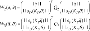
The proposed output-feedback adaptive control scheme is defined as

where q̄=q-qd for any constant (desired equilibrium position) vector qd∈Rn, G(q) is the regression matrix related to the gravity vector, according to Property 6, such that g(q,θ) = G(q)θ, KP∈Rnxn and KD∈Rnxn are positive definite diagonal matrices, i.e., KP=diag[kP1,…,kPn] and KD = diag[kD1,…,kDn] with kPi>0and kDi>0 for all i=1,…,n,

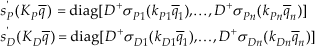
and
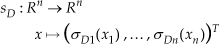
with σDi(·) and σDi(·), i = 1,…,n, being generalized saturation functions with bounds MPi and MDi such that

i = 1,…,n,3 ϑ ∈ Rn (the velocity estimator) and


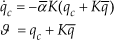
(the velocity estimation [or motion dissipation dynamic] algorithm)


(the parameter estimation [or adaptation] algorithm), where A ∈ Rnxn, B∈Rnxn and Γ∈Rpxp are positive definite diagonal matrices i.e., A = diag[ai,…,a n ] and B = diag[bi,…,bn], with ai>0 and bi>0 for all i = 1,…,n and Γ = diag[γ1,…,γr] with γ j >0 for all j = 1,…,p, qc and φc are the (internal) state vectors of the auxiliary dynamics in Eqs. (6a) and (7a) respectively, Y(q) is the regression vector related to the potential energy function, according to Property 6, i.e., U(q, θ) = Y(q)θ,

with σ aj (·), j=1,…,p, being strictly increasing generalized saturation functions with bounds Maj satisfying inequalities (3), α is a constant that may arbitrarily take any real value and e is a (sufficiently small) positive constant. A block diagram of the proposed output-feedback adaptive control scheme is shown in Fig 1.
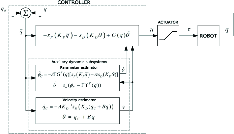
Block diagram of the proposed scheme
term was considered in a previous approach [18]. Furthermore, the α -term in (7a) has a natural influence in the closed-loop responses which could be used for performance adjustment purposes. This aspect is not explored in this work.
4. Closed-loop analysis
Consider system (1) and (2), taking

with φ*=(φ*1,…,φ*
p
)
T
, such that sa(φ*) = θ, or equivalently, φ*
j
= σ−1
aj
(θ
j
) j = 1,…,p. 4 Observe that from the satisfaction of inequalities (3) and (5), we have

Thus, under the consideration of Property 6 and the variable transformation (8), the closed-loop dynamics adopt the (equivalent) form5


where
while the parameter estimation error equilibrium vector
Let


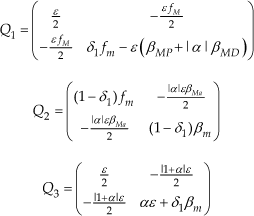
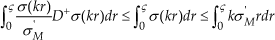
where
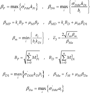
with σ PiM and σ DiM being the positive bounds of D+ σ Pi (·) and D+ σ Di (·) respectively, in accordance to point 2 of Lemma 1, and μ m , μ M , kc, fm, and fM as defined in Properties 1, 2 and 4. We are now ready to state the main analytical result.

where

and

with ε satisfying

Observe that from Property 1 and point 3 of Lemma 1, we have

where

with

and δ0 is a positive constant satisfying

(see (12)). Furthermore, note that, by (14),

where
Observe that from Properties 1, 2 and 4 and points (b) of Definition 1 and 2 of Lemma 1, we have

where

with
where δ1 is a positive constant satisfying

Let us note that the fulfilment of (12) guarantees the existence of values
5. Experimental results
In order to experimentally corroborate the efficiency of the proposed scheme, referred to as the SP-SDc-ga controller, real-time control implementations were carried out on a 3-DOF manipulator. The experimental setup, shown in Fig. 2, is a 3-revolute-joint anthropomorphic arm located at the Benemerita Universidad Autonoma de Puebla, Mexico. The actuators are direct-drive brushless motors (from Parker Compumotors) operated in torque mode, so they act as a torque source and accept an analogue voltage as a reference of torque signal. Position information is obtained from incremental encoders located on the motors. The setup includes a Pentium host computer and a system of electronic instrumentation, based on the motion control board MFIO3A, manufactured by Precision Microdynamics. The robot software is in open architecture, whose platform is based in C language to run the control algorithm in real time. The control routine registers data generated during the first 2000 samples at a default sample time of Ts = 2.5 ms, but Ts can be changed to higher values in accordance to the desired experimental duration. The experiments carried out in the context of this work, whose results are presented below, were run taking Ts= 0.12 s. A more detailed technical description of this robot is given in [30].

Experimental setup
For the considered experimental manipulator, Properties 5 and 6 are satisfied with


with q*∈U0={q∈R3:q2=q3=0}, i.e., such that U(q*,θ) = 0, ∀q*∈U0 (see Property 6). The maximum allowed torques (input saturation bounds) are T1 = 50 Nm, T2 =150 Nm and T3 =15 Nm for the first, second and third links respectively. From these data, one easily corroborates that Assumption 1 is fulfilled.
The involved saturation functions were defined as σ Pi (ς) = MPi sat (ς/MPi), σ Di (ς) = MDi sat(ς/MD), i=1,2,3, and

j=1,2, where

with 0 < Laj < Maj. Let us note that with these saturation functions we have σ
PiM
=σ
DiM
=1, ∀i∈ {1,2,3}.. The experimental implementations were run fixing the following saturation parameter values (all of them expressed in Nm): MP1 =MD1= 20, MP2 =MD2= 35, MP1=MD1= 4, Ma1=70, Ma2=5, and Laj=0.9Maj, j = 1,2. These saturation function parameter values were corroborated to satisfy inequalities (3) and (5), taking
For comparison purposes, additional experiments were run implementing the output-feedback adaptive algorithm proposed in [18], referred to as the L00 controller (choice made in terms of the analogue nature of the compared algorithms: output-feedback adaptive developed in a bounded input context; comparison of controllers of a different nature loses coherence), i.e.,

where Gd=G(qd), Th(x) = (tanh(x1),…,tanh(xn))
T
, K
P
∈R
n
and KD ∈ R
n
are positive definite diagonal matrices, λ and Δ are positive constants and
and

where K∈R n is a positive definite diagonal matrix and α, β, η and μ are positive constants. Arguing simplicity of development, the constant matrices involved in this control algorithm are taken in [18] as KP = kPIn, KD=kDIn and K = kIn, with kP, kD and k being positive constants. However, in order to speed up the closed-loop responses, different P and D control gains were considered at every input control expression. In other words, KP and KD in (17a) were taken as KP=diag[kP1,…,kPn] and KD = diag[kD1,…,kDn] with gains kPi and kDi, i =1,…,n, which each have their own different positive value. Furthermore, observe that through this controller, if input saturation is to be avoided, the control gains must satisfy saturation-avoidance inequalities of the form kPi+kDi ≤ Ti - Bi, i = 1,…,n, for some initial-condition-dependent positive constants Bi, i = 1,…,n.
The initial conditions and desired link positions for all the executed experiments were: q i (0) = q̇(0) = ϑi(0) = 0, qd1 = qd2 = π/4 and qd3 = π/2 [rad]. With this desired configuration, the condition stated by Corollary 1 turns out to be satisfied.7
For the proposed controller, with α = −1, the selected parameter combination was found through simulation tests, so as to have as good closed-loop responses as possible, mainly in terms of stabilization time (as short as possible) and transient response (avoiding or lowering down overshoot and oscillations as much as possible), and further refining the tuning experimentally. The resulting values were KP=diag[350, 400, 75] Nm/rad, KD=diag[25, 50, 12] Nms/rad, A=diag[15, 50, 35] rad/s2, B=diag[5, 10, 5] s−1, Γ = diag[5,0.5] Nm/rad and ε = 1.5 rad/Nms. As for the L00 controller, a similar tuning procedure was performed disregarding the saturation-avoidance inequalities in view of the considerably poor closed-loop performance observed under their consideration. The resulting values were: KP=diag[800, 1300, 200] Nm, KD=diag[5,10,10] Nm, λ = 30 [rad]−1, δ = 5 s/rad, k=50 s−1, η = 5, β = 25 Nm/rad, η = 5 rad/s and μ = 10 rad/s.
Figures 3–5 show the results for both implemented controllers. Observe that the regulation objective was achieved preventing input saturation and avoiding steady-state position errors. Furthermore, note that despite the presence of a small overshoot, through the SP-SDc-ga algorithm shorter stabilization times took place in both position error and parameter estimation responses. Let us further note that at 240s, where the experimental data registration was stopped, the parameter estimations were still evolving. This is a consequence of the slow evolution of the adaptation subsystem dynamics, due to the relatively small value of s in the proposed scheme and the analogue coefficients η and μ in the L00 controller. Nevertheless, the slow evolution of the adaptation subsystem dynamics did not have any influence on the position responses, which had been stabilized during the initial seconds of the experiment. The subsequent parameter estimator evolution was expected to reduce the difference among the estimations obtained through each implemented controller.

Position errors

Control signals

Parameter estimates
6. Conclusions
In this work, an output-feedback adaptive control scheme for the global regulation of robot manipulators with bounded inputs was proposed. With respect to the previous output-feedback adaptive approaches developed in a bounded-input context, the proposed velocity-free feedback controller guarantees the adaptive regulation objective: globally, avoiding discontinuities throughout the scheme, preventing the inputs from reaching their natural saturation limits and imposing no saturation-avoidance restriction on the control gains. Moreover, the developed scheme is not restricted to the use of a specific saturation function to achieve the required boundedness, but may rather involve any one within a set of smooth and non-smooth (Lipschitz-continuous) bounded passive functions that include the hyperbolic tangent and the conventional saturation as particular cases. The efficiency of the proposed scheme was corroborated through experimental tests on a 3-DOF manipulator. Good results were obtained, which were observed to improve those gotten through an algorithm that was previously developed in an analogue analytical context.
A Proof of Lemma 1
Since σ is a Lipschitz-continuous function that keeps the sign of its argument (according to point (a) of Definition 1) and is non-decreasing and bounded by M, there exists positive constants c < M and c+≤M such that

Hence, we have
Since σ is a Lipschitz-continuous non-decreasing function, D+σ(ς) exists and is piecewise-continuous on R and
From Lipschitz-continuity of σ, its satisfaction of point (a) of Definition 1 and the boundedness of D+σ by a positive constant σ M (according to point 2 of the statement), it follows that

∀ς∈R, whence (considering that σ has the sign of its argument, according to point (a) of Definition 1), we have
wherefrom we get

Strict positivity of
By the Lipschitz-continuous and non-decreasing characters of σ and its satisfaction of point (a) of Definition 1, there exist constants a > 0, ka > 0, and c≥1, such that |σ(ς)|≥ka\a sat(ς/a)| c , whence we get

∀ς∈R, with

Thus, from these expressions we can observe, on the one hand, that
Suppose σ is strictly increasing. Let Ψ,η,ς ∈ R. For any constant
Lipschitz-continuity. From the Lipschitz-continuity of σ and point 2 of the statement, we have
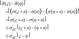
∀ς∈R which shows that
Strictly increasing monotonicity. From the strictly increasing monotonicity of σ, we have

which shows that
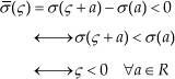
and

whence one sees that, for any

∀ς∈R
Thus, according to Definition 1,
B Theorem 7.2.1 of [29]
Theorem 7.2.1 in [29] states a version of La Salle's Invariance Principle that considers autonomous systems with continuous dynamics and makes use of continuous scalar functions and their upper-right derivative along the system trajectories (in contrast, for instance, with the statement presented in [24, Theorem 4.4], which is addressed to autonomous state equations with locally Lipschitz-continuous vector fields and makes use of continuously differentiable scalar functions). Consider the autonomous system

where f:D→R n is continuous, D⊂R n is an open connected set and f(0 n ). Theorem 7.2.1 in [29] is stated as follows.
The use of the upper right-hand derivative of V along the system trajectories, D+V, in the statement of this theorem, is corroborated in [29, §6.1A].
Footnotes
7. Acknowledgements
The first and third authors were supported by CONACYT, Mexico (3rd author: Project No. 134534). One of the authors, V. Santibáñez, thanks José A. Yarza for his invaluable help during the experimental essays.
1
The upper right-hand derivative D+φ is defined by
2
Property 5 is not satisfied by all types of robot manipulators but it is, for instance, by those with only revolute joints [2, Sect. 4.3]. This work is addressed to manipulators satisfying Property 5.
3
Observe that the satisfaction of inequalities (3) guarantees positivity of the right-hand side of inequality ![]() . As will become clear later, inequality (5) constitutes the tuning criterion on MPi and MDi through which the input variables ui are prevented from reaching their natural saturation bound Ti along the closed-loop trajectories.
. As will become clear later, inequality (5) constitutes the tuning criterion on MPi and MDi through which the input variables ui are prevented from reaching their natural saturation bound Ti along the closed-loop trajectories.
4
Notice that their strictly increasing character renders the generalized saturations σ aj , j = 1,…,p, (involved in the definition of sa) invertible.
5
6
See for instance [25, Chap. II, Sect. 6], where (generalized) statements of Lyapunov's second method are presented under the consideration of locally Lipschitz-continuous Lyapunov functions and their upper right-hand derivative along the system trajectories.