Sage Journals: Discover world-class research

Abstract

We present a novel vision servoing method, which is fit for climbing robots and those in unstructured environments, based on texture analysis. A large textured area is the target for observation. After the definition of texture element distribution density, the relationship between the change of the density at some selected points and the camera pose is deduced. The vision servoing control law, which meets the requirement of Lyapunov stability is designed in this paper. Experiments show the effectiveness of this method.

Keywords

Vision Servoing Texture Station Keeping Robot Vision Control

1. Introduction

Vision servoing is widely used in object tracking, grasping and robot station keeping. The image feature is a main aspect, which decides the controlling capability. Geometrical primitives, object contours, regions of interest, optical flow and the models of the tracked objects ^[1–7] are often employed. Edges and texture ^{[8, 9]} are the two major sources of visual features used in markerless visual tracking. For scenes with sharp edges or high spatial gradients, contour features are very informative. If illumination changes, edge information provides a good result in object tracking. If the scene is filled with texture and there is no obvious edge, contours may be absent. Texture-based methods are required in such situations ^[10]. Most of these methods at present are based on interesting points detection, where Harris corners are very popular. However, tracking interest points is sensitive to noise and changes in illumination. Some researchers integrated the texture and contour cues. Hafez ^[10] developed an integration framework that integrates edge and texture points for planar object visual tracking. After studying various illumination models that improve tracking robustness, Pressigout presented a hybrid contour and texture tracker that allows fast and robust tracking on planar and non-planar objects for augmented reality applications ^[11]. In [12] a method was introduced to estimate the Jacobian transform matrix using non-linear minimization of a unique criterion that integrates both the texture and the edge information of the tracked object. Chen developed a fuzzy controller to maintain the lighting level suitable for robotic manipulation and guidance in dynamic environments ^[13].

Most of the visual features used in the existing vision servoing algorithm are focused on the features of a small area or a target. However, in some environments the target plane may be large and be filled with texture with no obvious edge. Even the texture elements style on the planar object may be dynamic. If the texture elements are similar to each other or those elements change their appearance all the time, it is difficult to match interesting points or analyse the contours of the texture. Such kinds of environment are very common in robots working in areas such as the seabed, sea surface, desert, etc. The tasks of the robots include station keeping, auto landing, climbing and so on. A novel vision servoing method based on texture analysing is proposed in this paper. We do not extract or match any interesting points as most of the existing vision servoing methods do. The relationship between the texture features and the camera pose is deduced in this paper. A vision servoing control law, which meets the requirements of Lyapunov stability law, is designed. The texture feature we choose is the distribution density of the texture elements.

In Part 2, we define the distribution density of texture elements at a point in the texture plane and deduce the relationship between the distribution density of texture elements and the camera pose. In Part 3, we design the vision servoing control rule, which meets the requirements of Lyapunov stability law. In Part 4, we design some experiments to prove the effectiveness of the method.

2. Relationship between the distribution density of texture elements and the camera pose

We define three coordinate systems: 1) The world coordinate system O_wX_wY_wZ_w, with the origin point O_w being at a position in the workspace, 2) The camera coordinate system O_cX_cY_cZ_c with the origin point O_c, crossing the optical centre of camera lens and sitting on the axis Z_w and 3) Imaging plane coordinate system O_imgX_imgY_imgZ_img, with the origin point O_img being at the cross point of the camera imaging plane and the optical axis of the camera. O_imgX_img is parallel to the row direction of the pixels arrangement and O_imgY_img is parallel to the column direction of the pixels arrangement (as shown in Figure 1).

Figure 1.

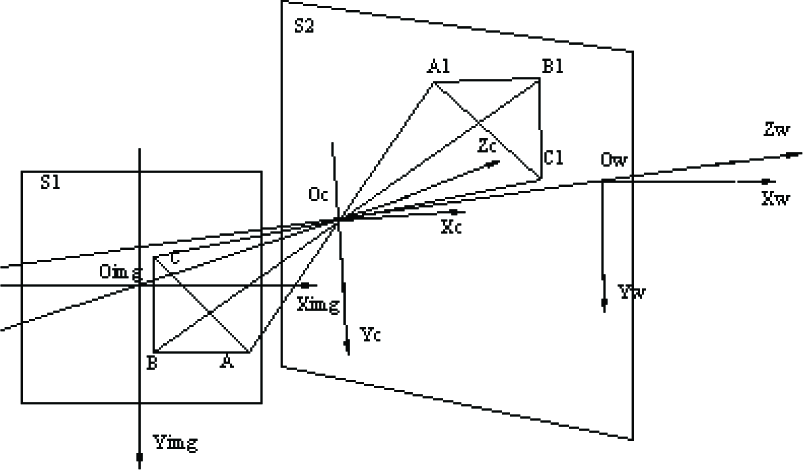
The sketch map of the texture elements density calculation

S1 is the camera imaging plane and S2 is the target texture plane observed by the camera. The plane equation for S2 in world coordinate systems is z_w = 0. The camera motion includes the rotation around axis O_c X_c, the rotation around axis O_cY_c and the translation along O_wZ_w.

Suppose P is a point in the world space. P is the coordinate of P in the camera coordinates system. ${\vec{P}}_{w}$ , which can be calculated by ${\vec{P}}_{w} = T R \cdot {\vec{P}}_{c}$ , is the world coordinate of $T R = T (Z ^{c}) \cdot R (X ^{c}) \cdot R (Y ^{c})$ (1) is the transformation matrix between the camera coordinates system and the world coordinates system. The translation order is: the camera coordinates and the world coordinates are coincident at the initial state. The camera coordinates system is moved along Z_c at the beginning and is then rotated around X_c, which follows the rotation around Y_c. T(Z_c), R(X_c) and R(Y_c) are the transformation matrices of the three motions respectively. Let z be the translation along Z_c, a be the rotation angle around X_c and bbe the rotation angle around Y_c. As shown in Figure 1, suppose A, B and C are the three non-collinear points in the image plane. Their coordinates in the camera coordinates system are:

\begin{array}{l} {\vec{A}}_{c} = {[x, y, - f, 1]}^{T}, {\vec{B}}_{c} = {[x - δ, y, - f, 1]}^{T} a n d \\ {\vec{C}}_{c} = {[x - δ, y - δ, - f, 1]}^{T} \end{array}

where f is the focal length of the camera and δ > 0 is a constant. A1, B1, C1 are the three corresponding points of A, B and C in the target plane. According to the solid geometry theory, the world coordinates ${\vec{A}}_{w}, {\vec{B}}_{w}, {\vec{C}}_{w}$ and ${\vec{O}}_{w}$ of the points A, B, C and O can be calculated using (1) respectively. For example, the world coordinates of point A are:

A_{w} = [\begin{matrix} x_{A w} \\ y_{A w} \\ z_{A w} \\ 1 \end{matrix}] = T R \cdot A_{c} = [\begin{matrix} x \cos b - f \sin b \\ x \sin a \sin b + y \cos a + f \sin a \cos b \\ - x \cos a \sin b + y \sin a - f \cos a \cos b + z \\ 1 \end{matrix}]

The calculations of ${\vec{B}}_{w}, {\vec{C}}_{w}$ and ${\vec{O}}_{w}$ are the same.

The area of triangle S_A1B1C1 is:

S_{A 1 B 1 C 1} = \sqrt{s_{A 1 B 1 C 1} (s_{A 1 B 1 C 1} - 1_{A 1 C 1}) (s_{A 1 B 1 C 1} - 1_{B 1 C 1}) (s_{A 1 B 1 C 1} - 1_{A 1 B 1})}

(1)

wheres s_A1B1C1=(l^A1C1+l_B1C1+l_A1B1)/2 and l_A1C1,l_B1C1 and l_A1B1 are the length of A1C1, B1C1, A1B1 respectively. Then the triangle area of A1B1C1 is:

S_{A 1 B 1 C 1} = δ^{2} z^{2} f ∕ (2 F 1 \cdot F 2 \cdot F 3)

(2)

where:

\begin{array}{l} F 1 = x \cos a \sin b - y \sin a + f \cos a \cos b \\ F 2 = x \cos a \sin b - δ \cos a \sin b - y \sin a + f \cos a \cos b \\ F 3 = x \cos a \sin b - δ \cos a \sin b - y \sin a + δ \sin a + f \cos a \cos b \end{array}

Suppose ρ is the texture element distribution density of a point in the target texture plane. It is obvious that all the texture elements in the triangle A1B1C1 will be imaged in the triangle ABC in the image plane. That means the amount of texture elements in A1B1C1 is equal to the amount of image points of the texture elements in ABC if one texture element in the image is considered as one point. Then the image points density of texture elements in triangle ABC is:

ρ S_{A 1 B 1 C 1} ∕ S_{A B C}

(3)

where:

S_{A B C} = δ^{2} ∕ 2

By substituting (2) into (3) and letting δ → 0, we get the texture element distribution density feature T of a point in the imaging plane, that is:

T = \lim_{δ \to 0} ρ S_{A 1 B 1 C 1} ∕ S_{A B C} = ρ z^{2} f ∕ {(x \cos a \sin b - y \sin a + f \cos a \cos b)}^{3}

(4)

where

x \cos a \sin b - y \sin a + f \cos a \cos b \neq 0 .

To prevent the conglutination of the texture elements in the image, the rotation angles of the camera are limited to (−π/4,π/4).

3. Designing of control law

3.1 Designing of Lyapunov function

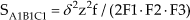
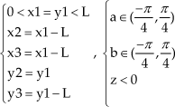
According to formula (4), suppose there are 3 points p1(x1,y1),p2(x2,y2) and p3(x3,y3) in the image plane, whose features can be calculated as formula (5):

{\begin{matrix} T 1 = \frac{ρ z^{2} f}{{(x 1 \cos a \sin b - y 1 \sin a + f \cos a \cos b)}^{3}} \\ T 2 = \frac{ρ z^{2} f}{{(x 2 \cos a \sin b - y 2 \sin a + f \cos a \cos b)}^{3}} \\ T 3 = \frac{ρ z^{2} f}{{(x 3 \cos a \sin b - y 3 \sin a + f \cos a \cos b)}^{3}} \end{matrix}

(5)

T1, T2 and T3 are all larger than or equal to 0 because of the physical meaning of texture distribution density. Ifp1(x1,y1),p2(x2,y2) and p3(x3,y3) are chosen following the rule shown in Figure 2, a unique solution of equation (5), as shown in (7), can be solved with the condition (6):

Figure 2.

Sketch map of choosing the appointed points for texture character calculation

{\begin{cases} 0 < x 1 = y 1 < L \\ x 2 = x 1 - L \\ x 3 = x 1 - L \\ y 2 = y 1 \\ y 3 = y 1 - L \end{cases}, {\begin{cases} a \in (\frac{- π}{4}, \frac{π}{4}) \\ b \in (\frac{- π}{4}, \frac{π}{4}) \\ z < 0 \end{cases}

(6)

{\begin{cases} a = \arctan [\frac{(x 3 - x 1 \cdot \sqrt[3]{\frac{T 1}{T 3}})] \cdot \sin b + f (1 - \sqrt[3]{\frac{T 1}{T 3}}) \cos b}{y 3 - y 1 \cdot \sqrt[3]{\frac{T 1}{T 3}}}] \\ b = \arctan {\frac{f [\sqrt[3]{\frac{T 1}{T 2}} \cdot (y 3 - y 1) + \sqrt[3]{\frac{T 1}{T 3}} (y 1 - y 2) - y 3 + y 2]}{\sqrt[3]{\frac{T 1}{T 2}} \cdot (x 3 \cdot y 1 - x 1 \cdot y 3) + \sqrt[3]{\frac{T 1}{T 3}} (x 1 \cdot y 2 - x 2 \cdot y 1) + x 2 \cdot y 3 - x 3 \cdot y 2}} \\ z = - \sqrt{\frac{1}{ρ f} {(x 1 \cdot \cos a \sin b - y 1 \cdot \sin a + f \cos a \cos b)}^{3} \cdot T 1} \end{cases}

(7)

Let the texture element distribution densities of the three points chosen above beT₁₀, T₂₀, T₃₀ respectively, when the camera is in its ideal position. If the camera pose changes, the distribution densities of the three points change toT, T₂ andT₃. Now an error function is defined as:

\vec{e} = {[e_{1}, e_{2}, e_{3}]}^{T} = {[T_{1} - T_{10}, T_{2} - T_{20}, T_{3} - T_{30}]}^{T} .

(8)

The task of vision servoing is to adjust the camera pose until function (8) reaches an accepted error ε.

The partial derivatives of the three points features with respect to a, b, z are:

\frac{\partial T_{i}}{\partial a}, \frac{\partial T_{i}}{\partial b}, \frac{\partial T_{i}}{\partial z}, i = 1, 2, 3.

(9)

From (5), the derivation result of the texture distribution density features of the chosen points with respect to t is:

\frac{d T_{i}}{d t} = \frac{\partial T_{i}}{\partial a} R_{a} + \frac{\partial T_{i}}{\partial b} R_{b} + \frac{\partial T_{i}}{\partial z} T_{r z}, i = 1, 2, 3

(10)

where $R_{a} = \frac{d a}{d t}$ is the rotation speed of the camera around

X_c, $X_{c}, R_{b} = \frac{d b}{d t}$ is the rotation speed of the camera around

Y_c and $T_{r z} = \frac{d z}{d t}$ is the translation speed of the camera along Z_w. Suppose the Lyapunov function is:

S = \frac{1}{2} \sum_{i = 1}^{3} {(T_{i} - T_{i 0})}^{2} .

(11)

There is only one solution (7) for function (5) under the condition (6). So the result of (11) will be 0 only when a = a₀, b = b₀ and z = z₀. Otherwise, it is larger than 0.

3.2 Designing of control law based on Lyapunov function

The derivation of the Lyapunov function (11) to the time t is:

\dot{S} = \sum_{i = 1}^{3} (T_{i} - T_{i 0}) \frac{d T_{i}}{d t} = \sum_{i = 1}^{3} Δ T_{i} \cdot (\begin{matrix} \frac{\partial T_{i}}{\partial a} & \frac{\partial T_{i}}{\partial b} & \frac{\partial T_{i}}{\partial z} \end{matrix}) {(\begin{matrix} R_{a} & R_{b} & T_{r z} \end{matrix})}^{T}, i = 1, 2, 3

(12)

If setting:

\frac{Δ T_{i}}{t} = - (\begin{matrix} \frac{\partial T_{i}}{\partial a} & \frac{\partial T_{i}}{\partial b} & \frac{\partial T_{i}}{\partial z} \end{matrix}) {(\begin{matrix} R_{a} & R_{b} & T_{r z} \end{matrix})}^{T}, i = 1, 2, 3

(13)

then:

\dot{S} = - t \sum_{i = 1}^{3} {[(\begin{matrix} \frac{\partial T 1}{\partial a} & \frac{\partial T 1}{\partial b} & \frac{\partial T 1}{\partial z} \end{matrix}) (\begin{matrix} R_{a} & R_{b} & T_{r z} \end{matrix})]}^{2} \leq 0

(14)

Because t>0, the equality exists only if:

\begin{array}{l} (\begin{matrix} \frac{\partial T_{1}}{\partial a} & \frac{\partial T_{1}}{\partial b} & \frac{\partial T_{1}}{\partial z} \end{matrix}) {(\begin{matrix} R_{a} & R_{b} & T_{r z} \end{matrix})}^{T} = (\begin{matrix} \frac{\partial T_{2}}{\partial a} & \frac{\partial T_{2}}{\partial b} & \frac{\partial T_{2}}{\partial z} \end{matrix}) {(\begin{matrix} R_{a} & R_{b} & T_{r z} \end{matrix})}^{T} \\ = (\begin{matrix} \frac{\partial T_{3}}{\partial a} & \frac{\partial T_{3}}{\partial b} & \frac{\partial T_{3}}{\partial z} \end{matrix}) {(\begin{matrix} R_{a} & R_{b} & T_{r z} \end{matrix})}^{T} = 0 \end{array}

This means ΔT₁ = ΔT₂ = ΔT₃ = 0 is valid only if (a = a₀ b = b₀ z = z₀)^T. Obviously the robot has moved to its ideal pose at this time. Otherwise, Ṡ < 0. Then the error function asymptotical converges to zero vectors.

3.3 Jacobian matrix and control law calculation

Change (13) to matrix style:

\frac{1}{t} [\begin{matrix} Δ T_{1} \\ Δ T_{2} \\ Δ T_{3} \end{matrix}] = - [\begin{matrix} \frac{\partial T_{1}}{\partial a} & \frac{\partial T_{1}}{\partial b} & \frac{\partial T_{1}}{\partial z} \\ \frac{\partial T_{2}}{\partial a} & \frac{\partial T_{2}}{\partial b} & \frac{\partial T_{2}}{\partial z} \\ \frac{\partial T_{3}}{\partial a} & \frac{\partial T_{3}}{\partial b} & \frac{\partial T_{3}}{\partial z} \end{matrix}] (\begin{matrix} R_{a} \\ R_{b} \\ T_{r z} \end{matrix}) = - J (\begin{matrix} R_{a} \\ R_{b} \\ T_{r z} \end{matrix})

(15)

where

J = [\begin{matrix} \frac{\partial T_{1}}{\partial a} & \frac{\partial T_{1}}{\partial b} & \frac{\partial T_{1}}{\partial z} \\ \frac{\partial T_{2}}{\partial a} & \frac{\partial T_{2}}{\partial b} & \frac{\partial T_{2}}{\partial z} \\ \frac{\partial T_{3}}{\partial a} & \frac{\partial T_{3}}{\partial b} & \frac{\partial T_{3}}{\partial z} \end{matrix}]

J is the Jacobian matrix, which shows the relationship between the changing speed of the image features and the camera motion speed. After calculation, we get:

| J | = \frac{18 ρ z^{5} f^{4} L^{2} \cos a}{G 1^{4} M 2^{4} M 3^{4}}

(16)

where:

\begin{array}{l} G 1 = x 1 \cos a \sin b - y 1 \sin a + f \cos a \cos b \\ M 2 = x 1 \cos a \sin b - L \cos a \sin b - y 1 \sin a + f \cos a \cos b \\ M 3 = x 1 \cos a \sin b - L \cos a \sin b - y 1 \sin a + L \sin a + f \cos a \cos b \end{array}

It is obvious that |J| ≠ 0 if the rule group (6) exists.

Then the inverse matrix J⁻¹ of J exists. If the two sides of (15) are multiplied by J⁻¹, we get:

(\begin{matrix} R_{a} \\ R_{b} \\ T_{r z} \end{matrix}) = - \frac{1}{t} {[\begin{matrix} \frac{\partial T_{1}}{\partial a} & \frac{\partial T_{1}}{\partial b} & \frac{\partial T_{1}}{\partial z} \\ \frac{\partial T_{2}}{\partial a} & \frac{\partial T_{2}}{\partial b} & \frac{\partial T_{2}}{\partial z} \\ \frac{\partial T_{3}}{\partial a} & \frac{\partial T_{3}}{\partial b} & \frac{\partial T_{3}}{\partial z} \end{matrix}]}^{- 1} [\begin{matrix} Δ T_{1} \\ Δ T_{2} \\ Δ T_{3} \end{matrix}] = - J^{- 1} \frac{1}{t} [\begin{matrix} Δ T_{1} \\ Δ T_{2} \\ Δ T_{3} \end{matrix}]

(17)

Formula (17) is the vision control law based on the texture element distribution density analysis.

4. Vision servoing experiments

A half physical experiment is designed to testify the availability of the proposed method. Large areas for observation are generated by a computer (4) and projected onto the screen (2) by the projector (3). A camera 1 is fixed in front of the screen and the images are captured by the calculation computer (4). The experiment environment is shown in Figure 3.

Figure 3.

Experiment environment

The parameters of the equipment are listed below:

1. Camera: MTV-188IEX, 2. White projector screen, 3. Projector: BENQ-PBL25XGA, 512*512 pixels, 4. Computer: Intel Core i5 2320 3.0GHz CPU, 4G memory, NVIDIA GTX470 display card, the programming tool is Visual C + +6.0. The control software interface is shown in Figure 4.

Figure 4.

Control software interface

The transform rule between the physical coordinates and the pixel coordinates should be given as follows:

x = (u - u 0) d x, y = (v - v 0) d y

(18)

where (u,v) are the pixel coordinates of an image point and (x,y) are the length coordinates. (u0,v0)are the pixel coordinates of the original point of the image plane. dx,dy are the distances between the two adjacent pixels in the directions of x, y respectively.

Image features are employed in the robot control in this method, which is not sensitive to the internal parameters error of the camera. â,b̂,ẑ (the estimation ofa,b,z) can be calculated when the internal parameters estimations of the camera are induced into (7). The motion speed of the camera in the pitching yawing and translation of the next step can be calculated when the parameters, including â,b̂,ẑ the estimation internal parameters of the camera, the distance of the features between the ideal position and the present position, are induced into (17).

Now we talk about the flow of control:

Set the estimated value of camera internal parameters û0,v̂0,dx̂,dŷ,f̂

Set the present and the ideal pose of the camera a,b,z,a0,b0,z0

Calculate the ideal density values at the three appointed points ${\vec{T}}_{0} = [\begin{matrix} T_{10} & T_{20} & T_{30} \end{matrix}]$

Calculate the present density values at the three appointed points $\vec{T} = [\begin{matrix} T_{1} & T_{2} & T_{3} \end{matrix}]$

Calculate the error between the values at the ideal and the present position $Δ \vec{T} = \vec{T} - {\vec{T}}_{0}$

If $∣ Δ \vec{T} ∣ > ε$ then go to 7) or else end the process

Calculate the speed values of the camera for the next step R_a, R_b, T_rz

Calculate the true value of the camera pose at present

{\begin{matrix} a = a + k a \cdot R_{a} \cdot t \\ b = b + k b \cdot R_{b} \cdot t \\ z = z + k z \cdot T_{r z} \cdot t \end{matrix}

9. Go to 4)

The control order sending period is set at 250ms. $\frac{1}{t} {[\begin{matrix} Δ T_{1} & Δ T_{2} & Δ T_{3} \end{matrix}]}^{T}$ is the changing speed of the image feature if t = 1 in (17). p in (17) is the only influence on the motion speed of the camera and proportional control is used, with the coefficients beingka,kb,kz. Then, ρ = 1 is suitable.

The real internal parameters of the camera are:

\begin{array}{l} u 0 = 245.2528066 \\ v 0 = 252.3415672 \\ d x = 0.009854238 \\ d y = 0.009851713 \\ f = 16. \end{array}

Some parameters are set as below. The pixel coordinates of the three chosen points in the texture image are:

\begin{array}{l} (u 1, v 1) = (462, 462) \\ (u 2, v 2) = (50, 462) \\ (u 3, v 3) = (50, 50) \end{array}

The ideal pose of the robot is:

a_{0} = - 5^{\circ}, b_{0} = 7^{\circ}, z_{0} = - 1000 m m .

The present pose of the robot is:

a = 20^{\circ}, b = - 20^{\circ}, z = - 700 m m .

The initial estimation internal parameters of the camera are:

\overset{⌢}{u} 0 = 256, \overset{⌢}{v} 0 = 256, \overset{⌢}{d} x = 0.009, \overset{⌢}{d} y = 0.009, \overset{⌢}{f} = 17.

The proportional control coefficients are:

k a = 0.5, k b = 0.5, k z = 1.

The experiment results are shown in Figure 5, where the horizontal axis shows the servoing time. The vertical axis shows the rotation angle or the amount of translation. The dotted line shows the ideal position of the camera.

Figure 5.

Curves of vision servoing process

A lot of similar experiments have been done with the same conditions. What's different to them is that the ideal poses and the present poses were changed to a different value each time. The results are similar to Figure 5. From the experiment results we can see that the robot can move to the ideal pose and position from the present pose and position with an acceptable error.

5. Conclusion and Discussion

It is difficult to use obvious geometry features such as corners, outlines, holes, etc. for robot visual servoing if the robot works in a textured environment. Geometry features in such environments are homogeneous, which is a big problem in robot control. The distribution density of the texture elements will change with some camera motions. With this cue, we develop this new method based on distribution density analysis. The shape or the contour of texture elements is not the feature used in this method. As a result, complex geometry structure matching or optical flow calculation, which can be an impossible mission in such environments, is not necessary. The main work is to calculate the distribution density of the texture elements at the different parts in the image. The most outstanding capability is that the method can be used in an environment with a dynamic textured surface. The reason is that the distribution density has nothing to do with the texture element shape or contour. Experiments showed an effective result.

However, there are some weaknesses to this method. First, vision servoing based on the distribution density of the texture elements is a statistical method. This means the control precision is not very high if the environment is filled with big texture elements and there is low density in a pointed area. The robot may swing with a small range at an ideal position when a high precision is requested. Second, big tilt angles of a robot are not allowed in this method because the texture elements that are far from the robot camera optical axis may conglutinate in the image with a big tilt angle. Last, this statistical method cannot deal with the motion of translation parallel to the camera image plane and the motion of rotation along with the optical axis. The reason is that the distribution densities in all the points in the view are similar at this time. A solution will come in future research by the author.

Although there are some shortcomings, as mentioned above, this new vision servoing method is still an effective theory. It solves a type of problem in robots control when working in a textured environment where there are no obvious geometric features.

References

Pressigout

Marchand

(2006) Real-time 3D Model-Based Tracking: Combining Edge and Texture Information. Proceedings of the 2006 IEEE International Conference on Robotics and Automation:2726–2731.

Kroger

Padial

(2012) Simple and Robust Visual Servo Control of Robot Arms using an On-lineTrajectory Generator. 2012 IEEE International Conference on Robotics and Automation:4862–4869

Anh

T. L.

Song

J. B.

(2012) Robotic grasping based on efficient tracking and visual servoing using local feature descriptors. International Journal of Precision Engineering and Manufacturing. 13(3): 387–393

Cui

G. Z.

Liang

K. K.

Guo

J. C.

(2012) A System of Robot Detecting and Tracking Moving Objects Based on Modified Optical Flow. Advances in Intelligent and Soft Computing. 169:259–265

Zang

C. T.

Hashimoto

(2012) A flexible Visual Inspection System Combining Pose Estimation and Visual Servo Approaches. 2012 IEEE International Conference on Robotics and Automation: 1304–1309

Chen

S. Y.

Y. F.

Kwok

N. M.

(2011) Active vision in robotic systems: A survey of recent developments. The International Journal of Robotics Research. 30(11):1343–1377

Zheng

W. W.

Zhu

Chen

S. Y.

(2012) Elman Fuzzy Adaptive Control for Obstacle Avoidance of Mobile Robots using Hybrid Force/Position Incorporation. IEEE Transactions on Systems, Man, and Cybernetics, Part C. 42(4):603–608.

Chen

C. H.

Huang

H. P.

S. Y.

(2011) Stereo-Based 3D Localization for Grasping Known Objects with a Robotic Arm System. Proceedings of the 8th World Congress on Intelligent Control and Automation:309–314.

Chen

S. Y.

(2012) Kalman Filter for Robot Vision: A Survey. IEEE Transactions on Industrial Electronics. 59(11):4409–4420.

10.

Hafez

Chari

Jawahar

C. V.

(2007) Combining Texture and Edge Planar Trackers based on a local Quality Metric. Proceedings of 2007 IEEE International Conference on Robotics and Automation:4620–4625.

11.

Pressigout

Marchand

(2005) Real Time Planar Structure Tracking for Visual Servoing: A Contour and Texture Approach. IEEE/RSJ International Conference on Intelligent Robots and Systems:251–256.

12.

Pressigout

Marchand

(2006) Hybrid Tracking Algorithms for Planar and Non-planar Structures Subject to Illumination Changes. Symp. on Mixed and Augmented Reality 06:52–55.

13.

Chen

Zhang

Kwok

N. M.

Y. F.

(2012) Intelligent Lighting Control for Vision-Based Robotic Manipulation. IEEE Transactions on Industrial Electronics. 59(8):3254–3263.

Vision Servoing Based on the Density Analysis of Texture Elements

Abstract

Keywords

1. Introduction

2. Relationship between the distribution density of texture elements and the camera pose

3. Designing of control law

3.1 Designing of Lyapunov function

3.2 Designing of control law based on Lyapunov function

3.3 Jacobian matrix and control law calculation

4. Vision servoing experiments

5. Conclusion and Discussion

References