Automated Trajectory Planner of Industrial Robot for Pick-and-Place Task

Abstract

Industrial robots, due to their great speed, precision and cost-effectiveness in repetitive tasks, now tend to be used in place of human workers in automated manufacturing systems. In particular, they perform the pick-and-place operation, a non-value-added activity which at the same time cannot be eliminated. Hence, minimum time is an important consideration for economic reasons in the trajectory planning system of the manipulator. The trajectory should also be smooth to handle parts precisely in applications such as semiconductor manufacturing, processing and handling of chemicals and medicines, and fluid and aerosol deposition. In this paper, an automated trajectory planner is proposed to determine a smooth, minimum-time and collision-free trajectory for the pick-and-place operations of a 6-DOF robotic manipulator in the presence of an obstacle. Subsequently, it also proposes an algorithm for the jerk-bounded Synchronized Trigonometric S-curve Trajectory (STST) and the ‘forbidden-sphere’ technique to avoid the obstacle. The proposed planner is demonstrated with suitable examples and comparisons. The experiments show that the proposed planner is capable of providing a smoother trajectory than the cubic spline based trajectory.

1. Introduction

Industrial robots, due to their great speed, precision and cost-effectiveness in repetitive tasks, now tend to be used instead of manual workers in automated production lines. These powerful machines are hardly autonomous, in the sense that they require preliminary actions such as calibration and trajectory planning in order to achieve defined tasks [1]. The trajectory planning problem is a fundamental one in robotics and defines a temporal motion law with a given geometric path, so that certain requirements set for the trajectory are fulfilled. The aim of trajectory planning is to generate the input for the control system of the manipulator to execute a motion. Figure 1 describes the structure of the automated trajectory planning system [2]. The input data for any trajectory planning algorithm are: geometric path, kinematic and dynamic constraints. The geometric path describes the path to be followed by the end-effector for continuous motion such as welding, painting, etc.; for a point-to-point motion such as a pick-and-place operation, however, the path of the end-effector is immaterial in the absence of obstacles. In the presence of any obstacles, the user defines the way point's position and the orientation of the end-effector or series of knot vectors to avoid the collision [3,4,5].

Figure 1.

Structure of automated trajectory planning system

The kinematic constraints are the velocity and acceleration limits (and jerk limits, if available) of the actuators as given by the manipulator manufacturer. Most of the manufacturers provide velocity limits for both joint-space motion and for task-space motion (i.e., straight-line path motion limits). The dynamic constraints specify torque limits for each joint. The high-level trajectory planner computes a reference trajectory for each task by checking the way points and assigns specific velocities to these points. The output is the trajectory of the joints (or of the end-effector), expressed as a time history of position, velocity and acceleration. Then, the completed portions of the trajectory are sent to the controller through a set-point generator. The proposed trajectory planner is able to generate a collision-free trajectory without any user-defined intermediate way points or knot points. This paper focuses on an automated trajectory planner for PUMA 560, the most-used industrial robot in experiments with 6-DOF, to carry out the pick-and-place operation.

Almost every technique found in the scientific literature on the trajectory planning problem is based on the optimization of some parameter or objective function. The general optimality criteria are: minimum execution time, minimum energy (or actuator effort) and minimum jerk. Some hybrid optimality criteria such as time-energy optimal trajectory planning and jerk time optimal trajectory planning have also been proposed. Minimum-time algorithms are tightly linked to the need to increase productivity in the industrial sector [4]. Pick-and-place is a non-value-added activity which at the same time cannot be eliminated. Hence, it must show minimal lead time and give maximum production. Therefore, the minimum time is considered to be important for economic reasons. However, in order to implement the trajectory in real time, the method must have a low computational complexity.

Jerk directly influences the motion of the robot in many aspects and a minimal jerk ensures smooth motion. The benefits of jerk minimization are: reduction in trajectory tracking errors, less stress induced in actuators and the structure of the manipulator, limited excitation of resonance frequencies of the robot, and the bringing about of natural and coordinated robot motion. It has been established that limiting jerk in manipulator trajectories reduces manipulator wear and improves tracking accuracy and speed [2,6-9]. Direct tracking of a time-optimal trajectory leads to joint vibrations and overshoot of the nominal torque limits [10]. Jerk limitation (and, proportionally, torque rate) results in smoothed actuator loads [6]. This effectively reduces the excitation of the resonant frequencies of the manipulator and consequently reduces actuator wear [9]. Low jerk trajectories can be tracked faster and more accurately [10]. Macfarlane and Croft [2] also inferred that a sine wave template for accelerations of smooth trajectory ensures that the quintics do not oscillate. Jerk minimization is considered as equal as or sometimes more than the minimum time requirement. Smooth motion without any unwanted variations in the manipulator's movement (i.e., with minimum jerk) is required for the applications such as semiconductor manufacturing, processing and handling of chemicals and medicines, fluid and aerosol deposition. On the above concerns, the generation of a smooth and minimum-time trajectory for a 6-DOF robot manipulator suitable for precise handling applications is the objective of the proposed trajectory planning system.

Various approaches have been attempted to obtain smooth and/or time-optimal trajectories. Initial work in robot trajectory planning focused mainly on time optimality [11]. Geering et al. [12] showed that the unconstrained time-optimal trajectory was either bang-bang or bang-singular-bang. Bobrow et al. [13] and Shin and McKay [14] showed that the optimal parameterized path to Path-Constrained Time-Optimal Motion (PCTOM) was also bang-singular-bang. It is further proved that all optimal paths must be saturated in at least one actuator at all times [15]. Kieffer et al. [16] developed a torque-based controller attempting to track the PCTOM while limiting actuator chatter. Constantinescu and Croft [10] presented a method for calculating smooth and time-optimal path-constrained trajectories. Smooth and time-optimal motion was obtained by optimizing a base trajectory subject to actuator torque and torque rate limits. Gasparetto and Zanotto [17] suggested an indirect method to get the same results, namely to set an upper limit on the jerk, defined as the time derivative of the acceleration of the manipulator joints. Cubic splines are often used in smooth trajectory generation [1518-27]. Since cubic splines can ensure the continuity of velocity and acceleration, they are widely used for interpolation and to prevent large oscillations of the trajectory, which can result in higher-order polynomials [18]. Cao et al. [25] optimized a piecewise cubic polynomial spline to obtain a smooth and time-optimal constrained motion. The time-optimal motion has been approximated using a Linear Segment with Parabolic Blends (LSPB) type trajectory with carefully selected switching points [10,13]. Chand and Doty [19] used polynomial splines to interpolate between joint target points. Higher order polynomials are generally not used due to their tendency to oscillate and, therefore, to generate retrograde motion [8,19]. Trigonometric Splines [26,28], Quintic Splines [2,4] and B-splines [29,30] have also been used to generate smooth trajectories. Various splines including the Cubic Spline, Trigonometric Spline, Polynomial Spline, Quintic Spline, B-spline are proposed for jerk-limited motion profiles. These profiles are generated with the help of knot vectors which are specified by the user for interpolation.

S-curve motion is another approach for jerk-limited motion [27-29]. The generation of S-curve trajectory does not require any knot points for interpolation. Tsay and Lin [27] developed an input strategy with fast acceleration and slow deceleration to minimize the residual response based on 3^rd order polynomial S-curve motion profiles. Nguyen et al. [28] presented the generalized polynomial S-curve model together with the proposal of a general algorithm to design S-curve motion trajectories. They also made a comparison of the actual velocity of the 3^rd, 4^th and 5^th order S-curve motions performed by the linear motor and the position errors of those S-curve motions. Their results indicate that the higher the order of the model, the better the performance of the linear motor. Experiments were also carried out on a linear motor system to study its performance with the motion profiles planned by the trigonometric model, which replaces the rectangular pulse in the jerk of the 3^rd order S-curve model by a trigonometric function. Li et al. [29] proposed acceleration-bounded S-curve motion for jerk-limited operation and implemented it on a Digital Signal Processing (DSP) based motion controller for a voice coil motor. The review reveals that the trigonometric S-curve trajectory is:

• as simple as the 3^rd order polynomial model and

• capable of producing a smooth trajectory as good as 5^th order polynomial S-curves and quintic splines.

Taking the above points into consideration, this paper proposes a new jerk-bounded S-curve trajectory with a sine wave form of jerk profile and the motion profiles: displacement, velocity and acceleration are generated within the maximum jerk value so as to obtain the desired smoother movement without any abrupt changes. This paper also proposes a trajectory planner for a smooth and minimum-time collision-free trajectory under kinematic and obstacle constraints for the pick-and-place operations of a 6-DOF robotic manipulator. The rest of the paper is organized as follows: section two describes the problem description, section three outlines the proposed planner with the illustrative numerical examples, section four discusses the results and section five presents the conclusion.

2. Problem Description

2.1 Operational features

Figure 2 shows the operation sequence of a 6-DOF robotic manipulator between two destinations. The robot's joints follow a Synchronized Trigonometric S-curve Trajectory (STST) between initial destination ‘P’ and final destination ‘Q’, which are described with Cartesian description. The STST has three phases: Acceleration, Constant Velocity and Deceleration.

Figure 2.

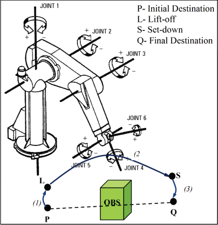
Operation sequence of a 6-DOF robotic manipulator between two destinations

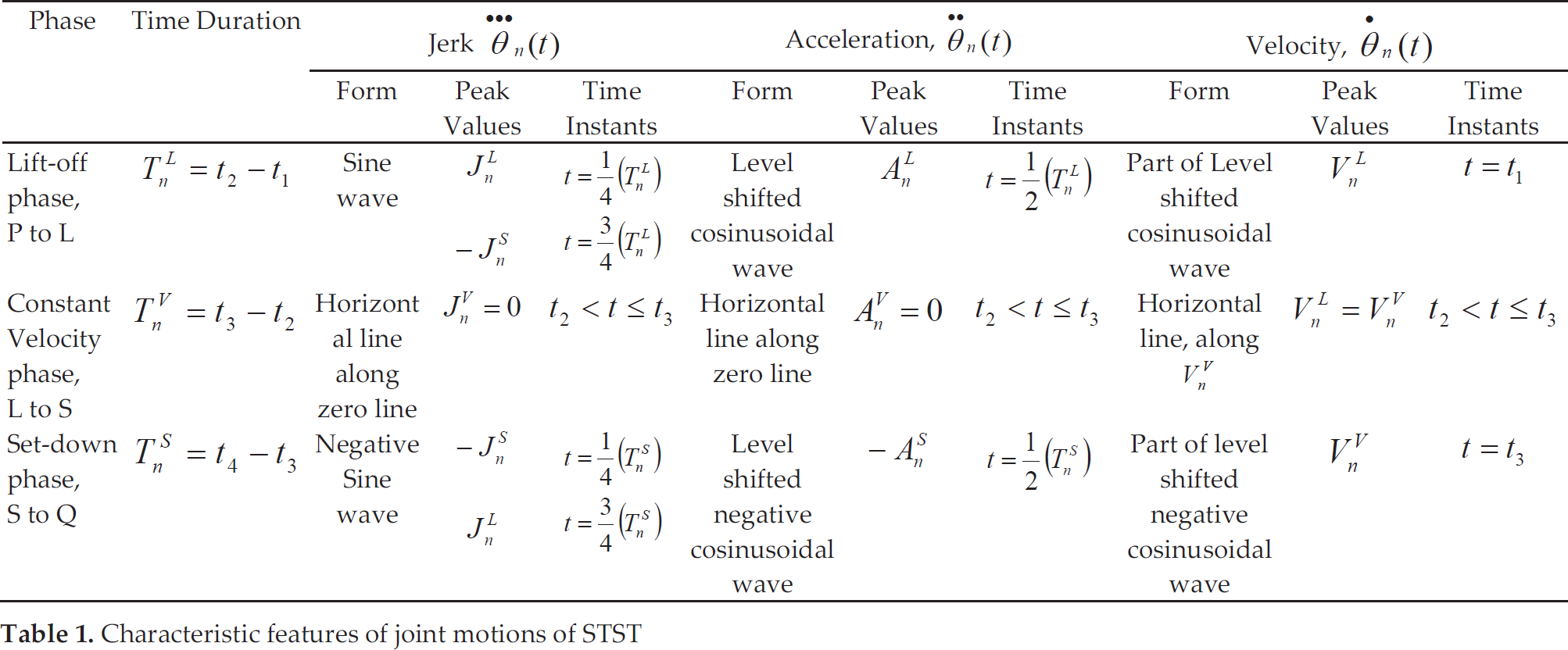
Let t₁, t₂, t₃ and t₄ be the absolute time instants when the robot is at the initial destination ‘P’, end of the acceleration phase ‘L’, start of the deceleration phase ‘S’ and final destination ‘Q’, respectively. Figure 3 shows the motion of each joint ‘n’ during the three phases, and the characteristic features are described in Table 1.

Table 1.

Characteristic features of joint motions of STST

Phase	Time Duration	Jerk ${\stackrel{̇̈}{\theta }}_n(t)$			Acceleration, ${\ddot{\theta }}_n(t)$			Velocity, ${\dot{\theta }}_n(t)$
		Form	Peak Values	Time Instants	Form	Peak Values	Time Instants	Form	Peak Values	Time Instants
Lift-off phase, P to L	TnL=t2 – t1	Sine wave	JLn – JSn	$\begin{array}{l}t=\frac{1}{4}\left(T_n^L\right)\hfill \\ t=\frac{3}{4}\left(T_n^L\right)\hfill \end{array}$	Level shifted cosinusoidal wave	AnL	$t=\frac{1}{2}\left(T_n^L\right)$	Part of Level shifted cosinusoidal wave	VnL	t = t1
Constant Velocity phase, L to S	TnV = t3 – t2	Horizont al line along zero line	JnV = 0	t2 < t ≤ t 3	Horizontal line along zero line	AnV = 0	t2 < t ≤ t3	Horizontal line, along VnV	VnL = VnV	t2 < t ≤ t3
Set-down phase, S to Q	TnS = t4 – t3	Negative Sine wave	– JSn JLn	$\begin{array}{l}t=\frac{1}{4}\left(T_n^S\right)\hfill \\ t=\frac{3}{4}\left(T_n^S\right)\hfill \end{array}$	Level shifted negative cosinusoidal wave	-AnS	$t=\frac{1}{2}\left(T_n^S\right)$	Part of level shifted negative cosinusoidal wave	VnV	t=t3

Figure 3.

Schematic Time History Trigonometric S-curve trajectory of a joint: a) Displacement, b) Velocity, c) Acceleration and d) Jerk

2.2 Objective criterion

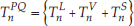
Generation of smooth trajectory for handling parts without vibration coupled with minimum time is the major objective under consideration in this paper. The proposed STST ensures jerk within the user-defined specifications. The minimum time depends on the sum of the time intervals during the three phases of the trajectory between the destinations ‘P’ and ‘Q’. Equation 1 provides the time taken by each joint to execute all the three phases.

$T_n^{PQ}=\left\{T_n^L+T_n^V+T_n^S\right\}$

(1)

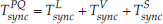
However, it is necessary that start and end instances of the three different phases of all the joints should occur at the same time to ensure the robot's end-effector follows an STST between any-destinations point ‘P’ and final destination ‘Q’. This is achieved by synchronizing all the joint motions with the joint that takes more time. Therefore, the execution time of the robot for the specified operation between the destinations ‘P’ and ‘Q’ is given in (2).

$T_{sync}^{PQ}=\left\{\underset{\forall n}{\max }\left(T_n^L\right)+\underset{\forall n}{\max }\left(T_n^V\right)+\underset{\forall n}{\max }\left(T_n^S\right)\right\}$

(2)

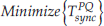
Hence, the objective function to the problem is the minimization of T^PQ_sync expressed in Equation (2).

2.3 Constraints

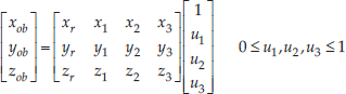
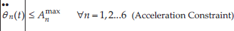
The robot kinematic parameters control/limit the minimum execution time and become the constraints on the problem. Each joint of the robot has its position within its specified range [θ_n^min, θ_n^max] and the kinematic constraints are: maximum velocity, V_n^max, maximum acceleration, A_n^max and maximum jerk J_n^max values of all (six) joints. Another important consideration in the trajectory planning problem is the presence of obstacles. This work considers the fixed obstacle (OBS) as a cube where side a and the reference base corner P_r are known. P₁, P₂ and P₃ are the extreme points on the obstacle along the X, Y and Z directions in relation to P_r as shown in Figure 4. With the help of these points, a set of parametrically discretized points of the obstacle is defined as R(x_ob, y_ob, z_ob), expressed in:

Figure 4.

Obstacle with its discretized set of points

$R(x_{ob},y_{ob},z_{ob})=P_r+u_1{P}_1+u_2{P}_2+u_3{P}_3$

(3)

where 0≤u₁,u₂,u₃≤1

where u₁, u₂, u₃ are the parametric variables of the X, Y and Z directions with respect to P_r. Figure 4 shows the discretized points of the obstacle. The above expression can also be written in a matrix form for the Cartesian components of the P_r, P₁, P₂ and P₃ as expressed in (4).

$\left[\begin{array}{c}{x}_{ob}\\ y_{ob}\\ z_{ob}\end{array}\right]=\left[\begin{array}{cccc}{x}_r& x_1& x_2& x_3\\ y_r& y_1& y_2& y_3\\ z_r& z_1& z_2& z_3\end{array}\right]\left[\begin{array}{c}1\\ u_1\\ u_2\\ u_3\end{array}\right]\begin{array}{cc}& 0\le u_1,u_2,u_3\le 1\end{array}$

(4)

In order to ensure the collision-free trajectory, interference of the end-effector or the links of the robot with the obstacle is to be avoided at all times. The joints of the robot have been considered as points and these points are connected by the line segments which represents the links of the robot. P_B, P_J1, P_J2, P_J3 and P_J4 are the Cartesian points of the robot base, joints 1, 2, 3 and 4, respectively. Since the origins of the other two joints 5 and 6 are located at the origin of joint 4, the robot is considered to have four links. The links are created parametrically as lines connecting the joints of the robot, i.e., line L₁ connecting P_B and P_J1 is link1 and other links L₂, L₃ and L₄ are similarly defined between PJ₁ and PJ₂, PJ₂ and PJ₃, and PJ₃ and PJ₄, respectively. The locations of robot joints and approximated links are specified in Figure 5, which depicts the link generation scheme and the zero position of the PUMA 560. Since the last three joints are intersected, the four links have been considered to represent the robot.

Figure 5.

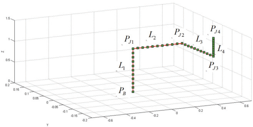
Link generation scheme for the robot configuration at zero position of PUMA 560

Let L(x,y,z,t) be the set of Cartesian points of these four lines, which represent the links of the manipulator at the time instant ‘t’. It is expressed in (5):

$L(x,y,z,t)=\left[\begin{array}{c}{L}_1\\ L_2\\ L_3\\ L_4\end{array}\right]=\left[\begin{array}{c}{P}_B\\ P_{J1}\\ P_{J2}\\ P_{J3}\end{array}\right]+u\left[\begin{array}{c}{P}_{J1}\\ P_{J2}\\ P_{J3}\\ P_{J4}\end{array}\right]\begin{array}{cc}& 0\le u\le 1\end{array}$

(5)

This restricts the free movement of the robot links and end-effector, and imposes an additional constraint.

2.4 Problem definition

The problem can be stated briefly thus:

“Determination of smooth (jerk-limited) and minimum-time trajectory of 6-DOF robotic manipulator, given the Cartesian position and orientation of end-effector at the pick-and-place destinations in its dexterous workspace, under the constraints of kinematic limitation on jerk, acceleration and velocity, and obstacle”.

2.5 Mathematical Model

The mathematical formulation is as follows:

Objective Function:

$Minimize\left\{T_{sync}^{PQ}\right\}$

(6)

Subject to

${\theta }_n^{\min }(t)\le {\theta }_n(t)\le {\theta }_n^{\max }(t)\begin{array}{cc}& \forall n=\mathrm{1,2...6}\end{array}\left(\text{Position\hspace{0.17em}Constraint}\right)$

(7)

$|{\stackrel{•}{\theta }}_n(t)|\le V_n^{\max }\begin{array}{cc}& \forall n=\mathrm{1,2...6}\end{array}(\text{Velocity\hspace{0.17em}Constraint)}$

(8)

$|{\stackrel{••}{\theta }}_n(t)|\le A_n^{\max }\begin{array}{cc}& \forall n=\mathrm{1,2...6}\end{array}\left(\text{Acceleration\hspace{0.17em}Constraint}\right)$

(9)

$|{\stackrel{•••}{\theta }}_n(t)|\le J_n^{\max }\begin{array}{cc}& \forall n=\mathrm{1,2...6}\end{array}\left(\text{Jerk\hspace{0.17em}Constraint}\right)$

(10)

$L(x,y,z,t)\not\subset R(x_{ob},y_{ob},z_{ob})(\text{Obstacle}\text{Constraint)}$

(11)

3. Proposed Trajectory Planner

The manipulator joint-level information has been considered for generating optimal trajectories in most contributions to the literature. However, offline programming requires defining the pick-and-place destinations with Cartesian space description. Taking this into consideration, the proposed planner is designed to execute smooth, time-optimal pick-and-place operations with the use of Cartesian description of end-effector at pick-and-place destinations without any user-defined intermediate way points or knot points. An enumerative procedure is proposed in pursuit of a smooth and minimum-time trajectory of a 6-DOF PUMA robot for handling fragile parts. The algorithm involves two stages: stage 1 searches for feasible trajectories without a via-point. Where there is no feasible solution in stage 1, the planner proceeds to stage 2 to search for feasible paths with a via-point. Figure 6 depicts the two-stage structure of the proposed planner. This section illustrates the different modules of the two-stage automated trajectory planner.

Figure 6.

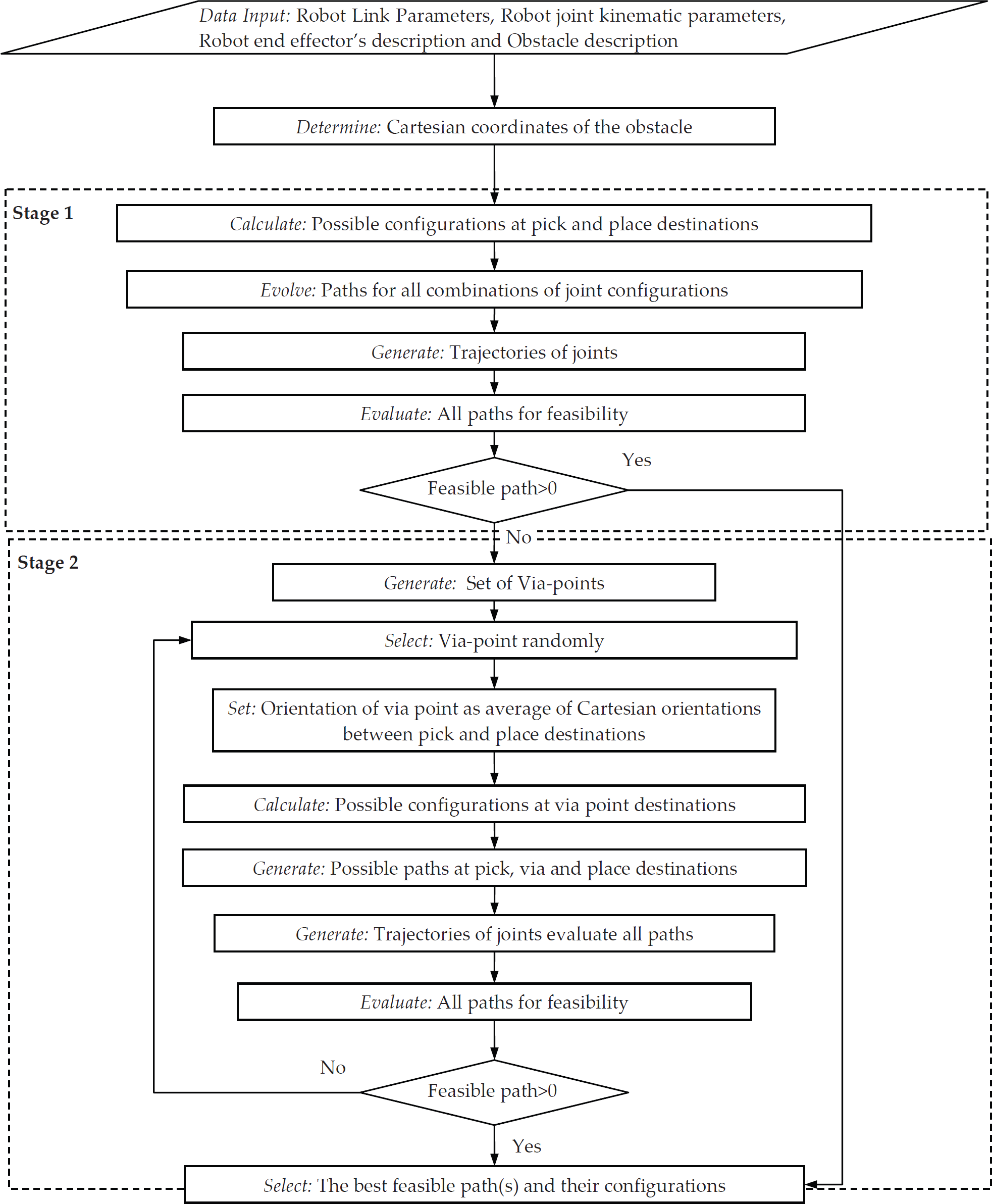
Flow chart of the proposed trajectory planner

3.1 Data Input

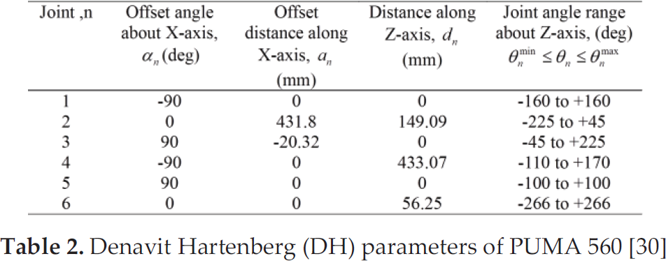
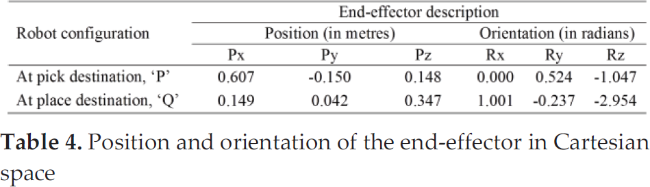
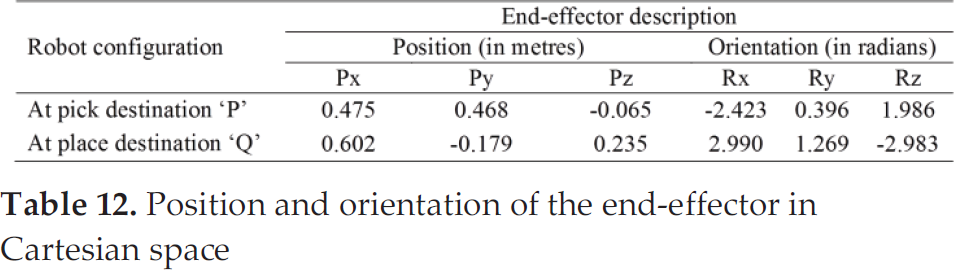
The data related to robot link and kinematic parameters, robot configurations at pick-and-place destinations, and the obstacle, are given as input. Consider the following data for illustration. The link parameters of PUMA 560 are shown in Table 2 [30] and its kinematic parameter limits are given in Table 3 [1]. Table 4 provides the position and orientations of the end-effector at pick-and-place destinations. The obstacle is assumed to be a cube of side 0.45 m and it is located with one of its base corners at a distance 0.2 m, 0 m and 0.8 m from the robot base.

Table 2.

Denavit Hartenberg (DH) parameters of PUMA 560 [30]

Joint,n	Offset angle about X-axis, an(deg)	Offset distance along X-axis, an (mm)	Distance along Z-axis, dn (mm)	Joint angle range about Z-axis, (deg) θnmin ≤ θn ≤ θnmax
1	−90	0	0	−160 to +160
2	0	431.8	149.09	−225 to +45
3	90	−20.32	0	−45 to +225
4	−90	0	433.07	−110 to+170
5	90	0	0	−100 to+100
6	0	0	56.25	−266 to +266

Table 3.

Kinematic parameters of PUMA 560

Kinematic Limits	Joint Description (Taken from [1])
	Joint 1	Joint 2	Joint 3	Joint 4	Joint 5	Joint 6
Velocity, Vnmax rad/s	8	10	10	5	5	5
Acceleration Anmax rad/s2	10	12	12	8	8	8
Jerk Jnmax rad/s3	30	40	40	20	20	20

Table 4.

Position and orientation of the end-effector in Cartesian space

	End-effector description
Robot configuration	Position (in metres)			Orientation (in radians)
	Px	Py	Pz	Rx	Ry	Rz
At pick destination, ‘P’	0.607	−0.150	0.148	0.000	0.524	−1.047
At place destination, ‘Q’	0.149	0.042	0.347	1.001	−0.237	−2.954

3.2 Determination of Cartesian coordinate of obstacle

When all parametric variables u₁, u₂, u₃ are zero, R (x_ob,y_ob,z_ob) represents the point P_r. If any one of these variables u₁,u₂,u₃ is one and other two variables are zero, R(x_ob,y_ob,z_ob) represents the extreme points P₁, P₂ and P₃ respectively. When all these variables reach their upper limit, one, then R(x_ob,y_ob,z_ob) denotes a corner of the cube which is diagonal to P_r. Therefore, a set of discretized points R(x_ob,y_ob,z_ob) is generated by varying each of the parametric variables whilst keeping the other two variables constant. In other words, each combination of the parametric variables provides a point on the obstacle. If each variable is incremented with 0.1 in all directions, this results in 1331 (11×11×11) points in the set R(x_ob,y_ob, z_ob).

3.3 Calculation of all eight possible configurations at the destinations

Given the Cartesian description of end-effector in dextrous workspace, there can be eight possible ways for a 6-DOF robotic manipulator to approach a particular destination through its inverse kinematic calculation. There are eight possible configurations as specified in the inverse kinematic solution tree for PUMA 560, as shown in Figure 7, at any Cartesian description of the end-effector in its dextrous workspace. The first three joints of PUMA 560 yield four possible positions with a combination of arm positions, ‘left’ and ‘right’ with ‘top’ and ‘down’, i.e., the first joint positions have four combinations of θ₁, θ₂ and θ₃, and their suffixes, ‘a’, ‘b’, ‘c’, and ‘d’, represent label of combination.

Figure 7.

Inverse kinematic solution tree for PUMA 560 robotic manipulator

Similarly, the wrist with θ₄, θ₅ and θ₆ has two kinds of orientation, ‘no flip’ and ‘flip’, for each combination of arm positions. The expressions (12), (13) and (14) show the relationship between wrist orientations ‘no flip’ and ‘flip’ [9]:

${\theta }_{5a}=-{\theta }_{5b}$

(12)

${\theta }_{4a}={\theta }_{4b}+{180}^{\circ }$

(13)

${\theta }_{6a}={\theta }_{6b}+{180}^{\circ }$

(14)

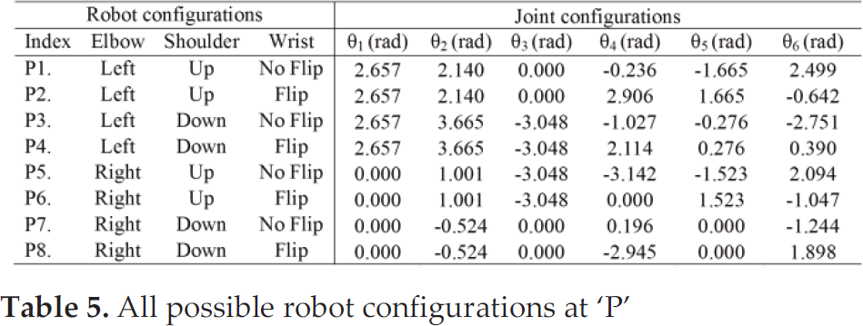
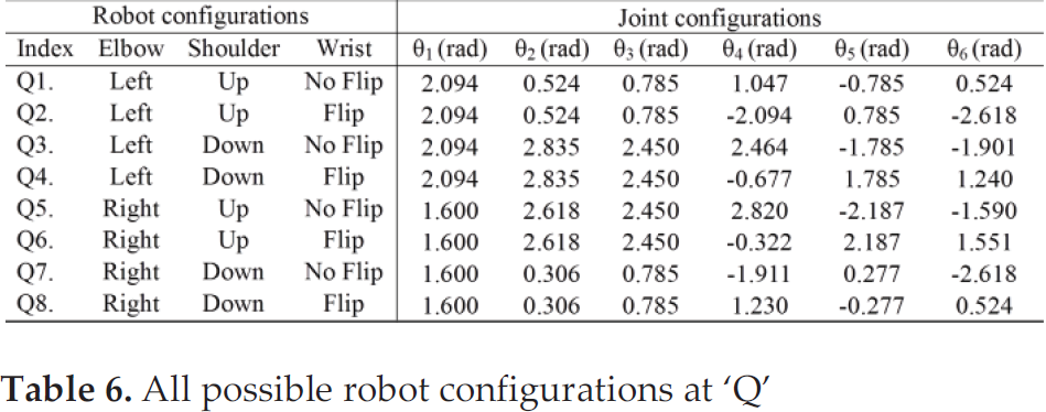
Table 5 and Table 6 provide the possible robot configurations at pick, ‘P’ and place, ‘Q’ destinations, respectively for the position and orientations of the end-effector as described in Table 4.

Table 5.

All possible robot configurations at ‘P’

Robot configurations				Joint configurations
Index	Elbow	Shoulder	Wrist	θ1(rad)	θ2(rad)	θ3(rad)	θ4(rad)	θ5(rad)	θ6(rad)
P1.	Left	Up	No Flip	2.657	2.140	0.000	−0.236	−1.665	2.499
P2.	Left	Up	Flip	2.657	2.140	0 000	2.906	1.665	−0.642
P3.	Left	Down	No Flip	2.657	3.665	−.1.048	−1.027	−0.276	−2.751
P4,	Left	Down	Flip	2.657	3.665	−.1.048	2.114	0.276	0.390
P5.	Right	Up	No Flip	0.000	1.001	−3.048	−3.142	−1.523	2.094
P6.	Right	Up	Flip	0.000	1.001	−3.048	0 000	1.523	−1.047
P7.	Right	Down	No Flip	0.000	−0.524	o.ooo	0.196	0.000	−1.244
P8.	Right	Down	Flip	o.ooo	−0.524	o.ooo	−2.045	0.000	1.898

Table 6.

All possible robot configurations at ‘Q’

Robot configurations				Join configurations
Index	Elbow	Shoulder	Wrist	θ1 (rad)	θ2 (rad)	θ3 (rad)	θ4 (rad)	θ5 (rad)	θ6 (rad)
Q1.	Left	Up	No Flip	2.094	0.524	0.785	1.047	−0.785	0.524
Q2.	Left	Up	Flip	2.094	0.524	0.785	−2.094	0.785	−2.618
Q3.	Left	Down	No Flip	2.094	2.835	2.450	2.464	−1.785	−1.901
Q4.	Left	Down	Flip	2.094	2.835	2.450	−0.677	1.785	1.240
Q5	Right	Up	No Flip	1.600	2.618	2.450	2.820	−2.187	−1.590
Q6	Right	Up	Flip	1.600	2.618	2.450	−0.322	2.187	1.551
Q7.	Right	Down	No Flip	1.600	0.306	0.785	−1.911	0.277	−2.618
Q8.	Right	Down	Flip	1.600	0.306	0.785	1.230	−0.277	0.524

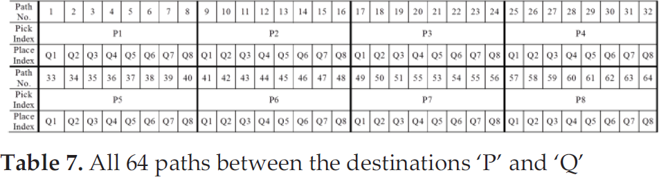
3.4 Generation of 64 possible paths for all combinations of joint configurations between destinations

Considering all combinations of robot configurations at pick-and-place destinations, there are 64 possible ways to move between destinations, i.e., combination of each robot configuration of ‘P’ with eight robot configurations of ‘Q’ results in 64 (8×8) paths between the destinations given in Table 7.

Table 7.

All 64 paths between the destinations ‘P’ and ‘Q’

Path No.	1	2	3	4	5	6	7	8	9	10	11	12	13	14	15	16	17	18	19	20	21	22	23	24	25	26	27	28	29	30	31	32
Pick Index	P1								P2								P3								P4
Place Index	Q1	Q2	Q3	Q4	Q5	Q6	Q7	Q8	Q1	Q2	Q3	Q4	Q5	Q6	Q7	Q8	Q1	Q2	Q3	Q4	Q5	Q6	Q7	Q8	Q1	Q2	Q3	Q4	Q5	Q6	Q7	Q8
Path No.	33	34	35	36	37	38	39	40	41	42	43	44	45	46	47	48	49	50	51	52	53	54	55	56	57	58	59	60	61	62	63	64
Pick Index	P5								P6								P7								P8
Place Index	Q1	Q2	Q3	Q4	Q5	Q6	Q7	Q8	Q1	Q2	Q3	Q4	Q5	Q6	Q7	Q8	Q1	Q2	Q3	Q4	Q5	Q6	Q7	Q8	Q1	Q2	Q3	Q4	Q5	Q6	Q7	Q8

3.5 Evolution and Evaluation of trajectories

This module generates STST, finds the execution time and checks for feasibility (i.e., collision-free) for all 64 paths. Figure 8 provides the sequence of steps involved, which are delineated in this section.

Figure 8.

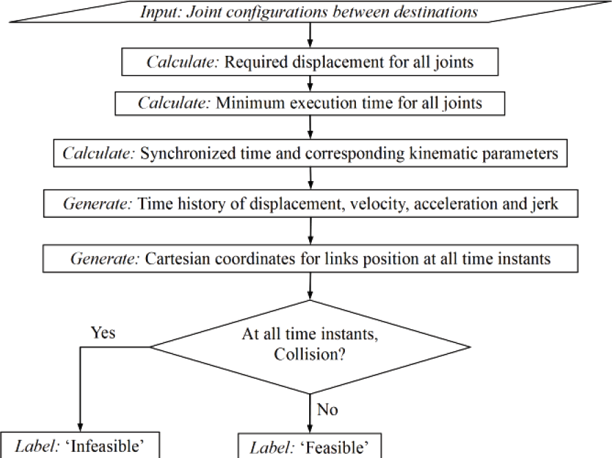
Flow chart of the feasible path generation module

3.5.1 Input: Joint configuration

The joint description (position and orientation) of the robot's joints θ^P_n and θ^Q_n at pick destination ‘P’ and place destination ‘Q’ is the input for the generation of STST. As an example, Table 8 provides the joint configuration of path no. 62 with its configurations P8 and Q6 at pick and place destinations respectively.

Table 8.

Data used for illustration of path no. 62

		θ1	θ2	θ3	θ4	θ5	θ6
Robot configuration	At pick destination (P8) θPn in rad	0.000	−0.524	0.000	−2.945	0.000	1.898
	At place destination (Q6) θQn in rad	1.600	2.618	2.450	−0.322	2.187	1.55

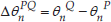
3.5.2 Calculation of required displacements for S-curve trajectory

Each joint requires a specific displacement Δθ_n^PQ for the move from ‘P’ to ‘Q’, and this is found using (15):

$\Delta {\theta }_n^{PQ}={\theta }_n{}^Q-{\theta }_n{}^P$

(15)

The required displacements of the joints for path no. 62 (Table 8) are:

$\begin{array}{l}\Delta {\theta }_n^{PQ}={\left[\Delta {\theta }_1^{PQ},\Delta {\theta }_2^{PQ},\Delta {\theta }_3^{PQ},\Delta {\theta }_4^{PQ},\Delta {\theta }_5^{PQ},\Delta {\theta }_6^{PQ}\right]}^{}\\ \hspace{0.17em}=\hspace{0.17em}\left[\mathrm{1.600,3.142,}\hspace{0.17em}\mathrm{2.450,}\hspace{0.17em}\mathrm{2.623,}\hspace{0.17em}\mathrm{2.187,}\hspace{0.17em}-0.347\right]\text{\hspace{0.17em}rad}\end{array}$

3.5.3 Calculation of minimum execution time and kinematic parameters of all joints

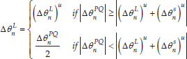
First, the lower bound of execution time is calculated. The kinematic parameters J_n^max, A_n^max, V_n^max limit the time for executing the motions during each of the three phases. The minimum time (T_n^L) ^l and its corresponding maximum displacement (δθ^L_n) during the acceleration phase are found using (16) and (17) respectively:

${\left(T_n^L\right)}^l=t_2-t_1=\frac{A_n{}^{\max }\pi }{J_n{}^{\max }}$

(16)

${\left(\Delta {\theta }_n^L\right)}^u=\frac{1}{4}{A}_n^{\max }\left({\left(T_n^L\right)}^2\right)$

(17)

Similarly, the minimum time (T_n^S) ^l and its maximum displacement (Δθ _n ^S ) _u during the deceleration phase are given in (18) and (19) respectively:

${\left(T_n^S\right)}^l=t_4-t_3==\frac{A_n{}^{\max }\pi }{J_n{}^{\max }}$

(18)

${\left(\Delta {\theta }_n^S\right)}^u=\frac{1}{4}{A}_n^{\max }\left({\left(T_n^S\right)}^2\right)$

(19)

The required displacement during the acceleration and deceleration phases are calculated as in (20) and (21):

$\Delta {\theta }_n^L=\{\begin{array}{cc}{\left(\Delta {\theta }_n^L\right)}^u& if|\Delta {\theta }_n^{PQ}|\ge |{\left(\Delta {\theta }_n^L\right)}^u+{\left(\Delta {\theta }_n^s\right)}^u|\\ \frac{\Delta {\theta }_n^{PQ}}{2}& if\left|\Delta {\theta }_n^{PQ}\right|<\left|{\left(\Delta {\theta }_n^L\right)}^u+{\left(\Delta {\theta }_n^s\right)}^u\right|\end{array}$

(20)

$\Delta {\theta }_n^S=\{\begin{array}{cc}{\left(\Delta {\theta }_n^S\right)}^u& if\left|\Delta {\theta }_n^{PQ}\right|\ge \left|{\left(\Delta {\theta }_n^L\right)}^u+{\left(\Delta {\theta }_n^s\right)}^u\right|\\ \frac{\Delta {\theta }_n^{PQ}}{2}& if\left|\Delta {\theta }_n^{PQ}\right|<\left|{\left(\Delta {\theta }_n^L\right)}^u+{\left(\Delta {\theta }_n^s\right)}^u\right|\end{array}$

(21)

The displacement during the constant velocity phase Δθ^V_n is calculated using (20) and (21) as given in (22):

$\Delta {\theta }_n^V=\{\begin{array}{cc}\Delta {\theta }_n^{PQ}-\Delta {\theta }_n^L-\Delta {\theta }_n^S& if\left|\Delta {\theta }_n^{PQ}\right|\ge \left|{\left(\Delta {\theta }_n^L\right)}^u+{\left(\Delta {\theta }_n^s\right)}^u\right|\\ 0& if\left|\Delta {\theta }_n^{PQ}\right|<\left|{\left(\Delta {\theta }_n^L\right)}^u+{\left(\Delta {\theta }_n^s\right)}^u\right|\end{array}$

(22)

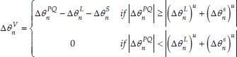
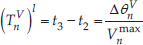
Therefore, the minimum time for the constant velocity phase is given in (23).

${\left(T_n^V\right)}^l=t_3-t_2=\frac{\Delta {\theta }_n^V}{V_n^{\max }}$

(23)

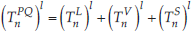
The minimum execution time of the joint ‘n’ during a robot motion cycle is given in (24):

${\left(T_n^{PQ}\right)}^l={\left(T_n^L\right)}^l+{\left(T_n^V\right)}^l+{\left(T_n^S\right)}^l$

(24)

Since the minimum time for the execution of the acceleration phase cannot be further reduced without increasing the jerk, the kinematic parameters A_n^max, J_n^max, V_n^max are to be adjusted/tuned to A^L_n, J^L_n and V_n^V for the required displacement, and are provided in (25), (26) and (28) respectively:

$A_n^L=\frac{4\Delta {\theta }_n^L}{{\left({\left(T_n^L\right)}^l\right)}^2}$

(25)

$J_n^L=\frac{A_n^L\pi }{{\left(T_n^L\right)}^l}$

(26)

The jerk and acceleration values will affect the velocity of each joint, calculated as in (27):

$V_n^L=\frac{{\left(A_n^L\right)}^2\pi }{2J_n^L}$

(27)

During the constant velocity phase, the acceleration and jerk are zero-valued, i.e., A^V_n = 0 and J_n^V = 0, and the velocity V_n^V equals the velocity limit of the acceleration phase V_n^L. It is kept constant throughout this phase.

$V_n^V=V_n^L$

(28)

The shape of the deceleration phase is symmetrical and has negative kinematic parameters. The Equations (29) and (30), respectively, provide the acceleration and jerk limits for the deceleration phase.

$A_n^S=\frac{4\Delta {\theta }_n^S}{{\left({\left(T_n^S\right)}^l\right)}^2}$

(29)

$J_n^S=\frac{A_n^S\pi }{{\left(T_n^S\right)}^l}$

(30)

Then, the velocity of the deceleration phase is calculated as in (31):

$V_n^S=\frac{{\left(A_n^S\right)}^2\pi }{2J_n^S}$

(31)

Considering the kinematic bounds as described in Table 2, the time and kinematic limits required for each joint in respect to the displacements are calculated using expressions (15) to (31) for an unsynchronized motion for the given input (Table 8). It is assumed that the time for both the acceleration and deceleration phases is equal, i.e., T^L_n = T_n^S. The time and corresponding kinematic parameters are calculated for all joints and tabulated in Table 9 as follows:

Table 9.

Time and kinematic information of unsynchronized motion for the 62^nd path

Parameters	Joints
	1	2	3	4	5	6
ΔθPQn (rad)	1.600	3.142	2.450	2.623	2.187	−0.347
(ΔθLn) u (rad)	2.742	2.665	2.665	3.158	3.158	3.158
ΔθLn (rad)	0.800	1.571	1.225	1.312	1.094	−0.174
TnL (sec)	1.047	0.942	0.942	1.2565	1.2565	1.2565
TnV (sec)	0	0	0	0	0	0
TnS (sec)	1.04/	0.942	0.942	1.2565	1.2565	1.2565
TnPQ (sec)	2.094	1.885	1.885	2.513	2.513	2.513
ALn (rad/sec2)	2.918	7.074	5.516	3.322	2.770	−0.439
JLn (rad/sec3)	8.754	23.582	18.388	8.305	6.925	−1.099
VVn = VLn (rad/sec)	3.056	6.668	5.199	−1.175	3.481	−0.552
ΔθSn (rad)	0.800	1.571	1.225	1.312	1.094	−0.174
ASn (rad/sec2)	−2.918	−7.074	−5.516	−3.322	−2.770	0.439
JSn (rad/sec3)	−8.754	−23.582	−18.388	−8.305	−6.925	1.099
VSn (rad/sec)	3.056	6.668	5.199	4.175	3.481	−0.552

3.5.4 Calculation of Synchronized execution time of S-curve trajectory and its kinematic joint limits

The trajectories are controlled by the combined acceleration and jerk values for the acceleration and deceleration phases. Specifically, these phases are influenced by the ratio of jerk and acceleration values. When jerk reaches its maximum bound, the ratio of jerk to acceleration is considered to be the trajectory frequency ω^L_n with which the pattern of trajectory of each kinematic parameter will be set, given in (27).

${\omega }_n^L=\frac{2J_n^L}{A_n^L}$

(32)

The trajectory frequency of the acceleration phase for the values given in Table 9 is: ω^L_n = [6.000 6.667 6.667 5.000 5.000 5.000] (cycles/sec).

Similarly to the acceleration phase, the deceleration phase of the trajectory has the frequency ω^S_n, which is given in (33):

${\omega }_n^S=\frac{2J_n^S}{A_n^S}$

(33)

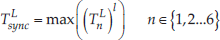
Since the times for the acceleration and the deceleration phases are equal (T_n^L = T_n^S) for the values given in Table 9, the trajectory frequency of the deceleration is ω^L_n, i.e., ω^S_n = [6.000 6.667 6.667 5.000 5.000 5.000] (cycles/sec). However, the motions of all joints during each phase should be time-synchronized for the robot to reach ‘L’ and ‘S’ points at the time instants t₂ and t₃ with STST. Synchronization means that the execution of the required displacement of each phase of motion of all joints is accomplished with the same start and end times. The kinematic parameters can be further reduced by synchronizing the motions of all joints with the slowest joint, the joint with the highest minimum execution time. In order to synchronize the joint motions, the execution times of three phases are calculated based on the slowest joint in their respective phases using (34) to (36).

$T_{sync}^L=\max \left({\left(T_n^L\right)}^l\right)\begin{array}{cc}& n\in \left\{\mathrm{1,2...6}\right\}\end{array}$

(34)

$T_{sync}^V=\max \left({\left(T_n^V\right)}^l\right)\begin{array}{cc}& n\in \left\{\mathrm{1,2...6}\right\}\end{array}$

(35)

$T_{sync}^S=\max \left({\left(T_n^S\right)}^l\right)\begin{array}{cc}& n\in \left\{\mathrm{1,2...6}\right\}\end{array}$

(36)

Then, total execution time for pick and place task is calculated as in (37).

$T_{sync}^{PQ}=T_{sync}^L+T_{sync}^V+T_{sync}^S$

(37)

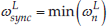
Therefore, other joints are operated with lesser kinematic values in order to synchronize their motion and for executing the smooth motion. In this work, it is considered that all the phases of the trajectory (acceleration, constant velocity and deceleration phases) are synchronized i.e. all joints execute the same phase of the trajectory at any instant of time. In order to synchronize all the joints, the synchronized trajectory frequency ω^L_sync is set as minimum value among the trajectory frequencies of the joints and is expressed in (38).

${\omega }_{sync}^L=\min \left({\omega }_n^L\right)$

(38)

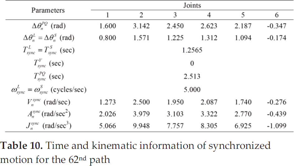
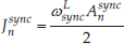
It is assumed that acceleration and deceleration phases operate with equal time interval T^L_sync = T^S_sync and hence, they have same trajectory frequency, i.e. ω^L_sync = ω^S_sync. The resultant the kinematic values during the acceleration and deceleration phases, are equal in their magnitude but differ in the sign. Then, the kinematic parameters (acceleration A_n^sync, jerk J_n^sync and velocity V_n^sync) are updated for synchronization with the help of the synchronized trajectory frequency ω^L_sync as given in (39), (40) and (41), respectively. The synchronized motion for the inputs given in Table 8 can be achieved through the expressions (34) to (41) and are given in Table 10.

Table 10.

Time and kinematic information of synchronized motion for the 62^nd path

Parameters	Joints
	1	2	3	4	5	6
ΔθPQn (rad)	1.600	3.142	2.450	2.623	2.187	−0.347
ΔθLn = ΔθSn (rad)	0.800	1.571	1.225	1.312	1.094	−0.174
TLsync = TSsync (sec)			1.2565
TVsync (sec)			0
TPQsync (sec)			2.513
ωLsync = ωSsync (cycles/sec)			5.000
Vnsync (rad/sec)	1.273	2.500	1.950	2.087	1.740	−0,276
Ansync (rad/sec2)	2.026	3.979	3.103	3.322	2.770	−0.439
Jnsync (rad/sec3)	5.066	9.948	7.757	S.305	6.925	−1.099

$A_n^{sync}=\frac{4\Delta {\theta }_n^L}{{\left(T_{sync}^L\right)}^2}$

(39)

$J_n^{sync}=\frac{{\omega }_{sync}^L{A}_n^{sync}}{2}$

(40)

$V_n^{sync}=\frac{A_n^{sync}\pi }{{\omega }_{sync}^L}$

(41)

3.5.5 Generation of time history of kinematic parameters of all joints for the synchronized motion

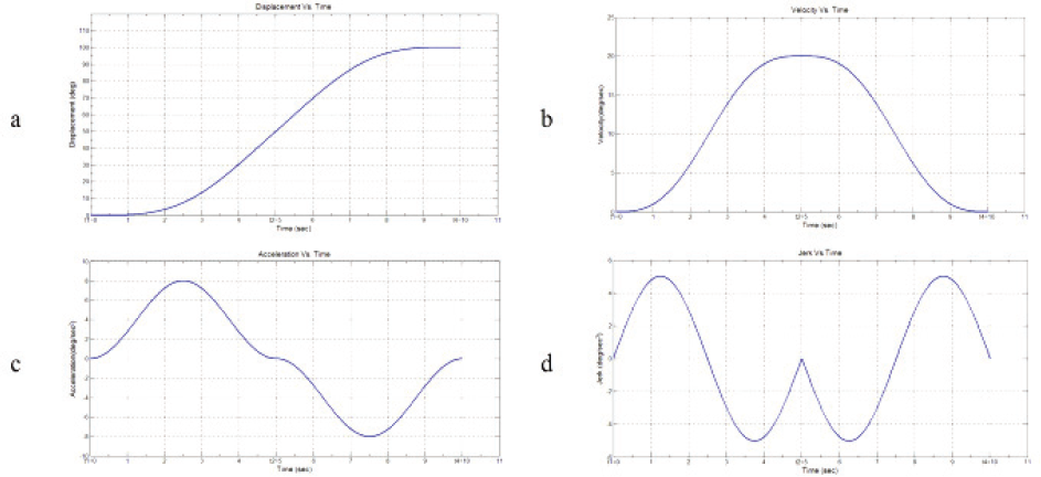
Once, the kinematic limits are identified, the time history (trajectory) of each kinematic parameter is generated for synchronized motion of the robot in carrying out the pick-and-place operation. Time history of joints may be with or without a constant velocity phase. For example, consider the following: θ₁ ^P = 0deg and θ₁ ^Q = 100deg are joint positions at initial destination ‘P’, and final destination ‘Q’, respectively, and whose maximum kinematic limits are V₁^max =10deg/sec; A₁^max = 4deg/ sec²; J₁^max = 2.5deg/sec³. Figure 9 depicts the time history of STST with the constant velocity phase generated using the expressions (15) to (31).

Figure 9.

Time history of joint (with constant velocity phase): a) Displacement, b) Velocity, c) Acceleration, d) Jerk

If the maximum kinematic limits of the joint are V₁^max = 20deg/ sec; A₁^max = 8deg/ sec²; J₁^max = 5deg/ sec³ with the same joint positions at ‘P’ and ‘Q’, then the corresponding STST is generated without the constant velocity phase, as shown in Figure 10.

Figure 10.

Time history of joint (without constant velocity phase): a) Displacement, b) Velocity, c) Acceleration, d) Jerk

With the help of the expressions for synchronization (15) to (41) and by operating at kinematic values given in Table 3, the STST for the configurations of the 62^nd path are generated and are shown in Figure 11. The time for executing the path between these configurations given in Table 8 is 2.513 sec and minimum of maximum jerk value is 9.9485 rad/sec³.

Figure 11.

STST of PUMA 560 for 62^nd path: a) Displacement, b) Velocity, c) Acceleration, d) Jerk

3.5.6 Generation of Cartesian coordinates for links at all time instants

With the help of the trajectory that has been generated in joint space, the Cartesian coordinate values of the links have been calculated/generated at every time instant of the synchronized motion. For the known robot joint space information, the Cartesian coordinate values of the joints are calculated using suitable transformation matrices of the forward kinematics, as described in section 2.3. The information on the links has been updated at every STST time instant.

3.5.7 Simulation of Collision check

In a working environment with an obstacle as shown in Figure 12, the synchronized trajectories generated in section 3.5.5 may be feasible, i.e., collision-free (represented by the continuous line) or infeasible (represented by the dotted line). For the known joint configurations at every instant of time, the path of the end-effector is generated with the help of forward kinematics. In order to generate a feasible trajectory, a collision check procedure is proposed between the links and the obstacle at all time instants of synchronized time during the robot's operation.

Figure 12.

Schematic sketch of robot positions in its trajectory

The path that is generated between the robot configurations of the destinations is evaluated for interference/collision of links with the obstacle and is labelled as ‘feasible’ or ‘infeasible’. Cartesian coordinate values of these links L(x,y,z,t) as generated in section 2.3 are compared with the Cartesian coordinate values of the obstacle R(x_ob, y_ob, z_ob); the difference between these Cartesian values should be greater than 0.01 m (assuming that the maximum thickness of the links of the robot is approximately 0.01 m) along X, Y and Z directions at all time instants. If the difference is less than 0.01 m, it indicates that the link has a contact with the obstacle and the corresponding path is labelled as ‘infeasible’. Otherwise, the collision check procedure will be evaluated for the next time instant and this process will be continued throughout the synchronized execution time T^PQ_sync. The successful path in the collision check will be labelled as ‘feasible’. In order to reduce the algorithm's computational effort, once collision is detected at any time instant, the proposed algorithm will exit immediately from the time loop, avoiding unwanted computations. Path no. 62, presented in section 3.5, has been labelled as ‘infeasible’ after the collision check, i.e., the robot makes contact with the obstacle during its motion along this path. All paths are evaluated and labelled in this way. Table 12 provides the execution time, maximum jerk and feasibility status of 64 paths generated by the algorithm.

Table 11.

Results of the algorithm for 64 possible paths from Cartesian space description

Path No.	Pick Configuration	Place Configuration	Execution Time (sec)	Jerk Limit (rad/sec3)	Feasibility Status
1	P1	Q1	2.51	6.255	Feasible
2	P1	Q2	2.51	16.201	Fungible
3	P1	Q3	2.51	13.932	Feasible
..	..	..	..		..
16	P2	Q8	2.51	6.151	Feasible
..	..	..	..
30	P4	Q6	2.53	16.871	Feasible
..	..	..	..
46	P6	Q6	2.53	16.871	Feasible
..	..	..	..
62	P8	Q6	2.51	9.9485	Infeasible
63	P8	Q7	2.51	14.297	hi feasible
64	P8	Q8	2.51	13.215	Infeasible

Table 12.

Position and orientation of the end-effector in Cartesian space

Robot configuration	End-effector description
	Position fin metres)			Orientation (in radians)
	Px	Py	Pz	Rx	Ry	Rz
At pick destination ‘P’	0.475	0.468	−0.065	−2.423	0.3%	1.986
At place destination ‘Q’	0.602	−0.179	0.235	2.990	1.269	−2.983

3.5.8 Selection of best feasible path and configurations

It is found that 48 feasible solutions (paths) are available among 64 solutions. The best feasible solution is selected based on minimum execution time and minimum jerk value. The path number 16 with pick-and-place configurations, P2 and Q8 respectively, whose path time of 2.513 sec and minimum of maximum jerk value of 6.151 rad/sec³ represent the best solution for the input given in section 3.1. This is the only path with both minimum time and minimum jerk value. The torque values have been calculated using Robotics Toolbox [31] to understand the dynamic behaviour of this proposed trajectory for the feasible paths.

Figure 13 depicts the corresponding trajectories of displacement, velocity, acceleration, jerk and torque for the optimal solution, i.e., trajectories for all the joints of PUMA 560 robot during its motion along path no. 16 with configuration P2 and Q8.

Figure 13.

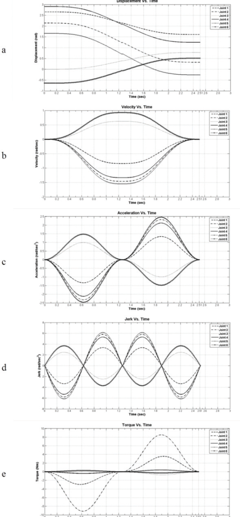
STST of PUMA 560 for the optimal path (path no. 16) among 64 paths: a) Displacement, b) Velocity, c) Acceleration, d) Jerk e) Torque

3.6 Generation of feasible trajectories with via-point

When all the 64 paths become ‘infeasible’ for the particular input, stage two of the planner searches for feasible path(s) between the pick and place destinations with a via-point.

In order to illustrate the above case, the data on the end-effector given in Table 12 have been considered without any change in robot link parameters and using kinematic limits as specified in Tables 2 and 3.

The obstacle that is considered is a cube of side 0.4 m with one of its base corner is located at a distance 0.2 m, 0 m and 0.8 m from the robot base in Cartesian space. For the above-given input to the algorithm, initially the following steps are executed as per the procedures presented in section 3.2 to 3.5 and the results of stage one. After evaluating 64 paths in collision check, it is found that all the paths are labelled as ‘infeasible’; this shows that along all the 64 paths the robot's links collide with the obstacle.

3.6.1 Selection of the via point for feasible trajectory generation

Under circumstances where all 64 paths generated from the Cartesian description of the end-effector fail, a via-point ‘V’ is needed to obtain a feasible path. The following procedure is proposed in this work to select a ‘via-point’ ‘V’ in the robot's dexterous workspace to generate a collision-free path.

3.6.1.1 Generation of forbidden sphere

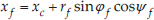
The work proposes a ‘forbidden sphere’ technique for the selection of via-point to generate a feasible trajectory. A forbidden enclosing sphere connecting the corners of cube (the obstacle) is developed which encapsulates the obstacle. The centre of the forbidden sphere P_c(x_c,y_c,z_c) and its radius ‘r_f’ are calculated from P_r (x_r,y_r,z_r), the Cartesian position of the reference base corner of the cube, and are given as in (42), (43) (44) and (45):

$x_c=x_r+a/2$

(42)

$y_c=y_r+a/2$

(43)

$z_c=z_r+a/2$

(44)

$r_f=\frac{\sqrt{3}}{4}a$

(45)

The points on the surface of the forbidden sphere (x_f,y_f,z_f) are calculated using its spherical coordinates (r_ƒφ_ƒφ_ƒ) and their corresponding expressions are given in (46), (47) and (48):

$x_f=x_c+r_f\sin {\phi }_f\cos {\psi }_f$

(46)

$y_f=y_c+r_f\sin {\phi }_f\sin {\psi }_f$

(47)

$z_f=z_c+r_f\cos {\phi }_f$

(48)

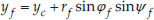
where 0 ≤ φ_f ≤ ∂ and 0 ≤ φ_f ≤ 2∂

3.6.1.2 Generation of via-point sphere

A set of three via-point spheres concentric to the forbidden sphere (sphere encompasses the obstacle) has been constructed to facilitate the selection of a via-point which emulates the workspace of the articulated robotic manipulator (a partial sphere in shape). Figure 14 depicts the arrangement of forbidden sphere and via-point sphere (only one via-point sphere has been shown for ease of understanding). A via-point sphere is generated from the centre of the forbidden sphere, i.e., P_c(x_c,y_c,z_c) and its calculated radius ‘r_v’, as given in (49):

Figure 14.

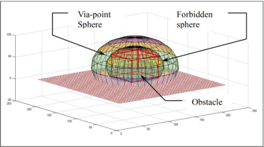
Via-point generation for obstacle avoidance

$r_v=r_f+offset$

(49)

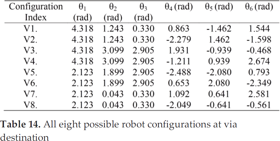
Two more via-point spheres are generated with the multiples of the same offset distances. Offset value is selected in such a way that the via-point spheres fall in the robot's dexterous workspace. Each sphere has been discretized to have 200 Cartesian coordinate points. All the points on the via-point spheres are stored as R(x_v,y_v,z_v), the pool of points for via-point selection. The trajectory planner selects a via-point randomly as required from a look-up table R(x_v,y_v,z_v). This selected via-point is considered as the Cartesian position of the end-effector and its orientation is assumed to be the average of the orientations at the pick-and-place destination. Position and orientation form the required transformation matrix which provides the Cartesian description at ‘V’. Table 13 presents the position and orientation of one such selected via-point and its corresponding transformation matrix. Similar to pick-and-place destinations, the possible configurations at a selected via-point destination is given in Table 14.

Table 13.

Position and orientation of the end-effector for the selected via-point

Robot configuration	End-effector description
	Position (in metres)			Orientation (in radians)
	Px	Py	Pz	Rx	Ry	Rz
At via-point destination	−0.026	0.328	0.428	0.284	0.833	−0.498

Table 14.

All eight possible robot configurations at via destination

Configuration Index	θ1(rad)	θ2(rad)	θ3(rad)	θ4(rad)	θ5(rad)	θ6(rad)
V1.	4.318	1.243	0.330	0.863	−1.462	1.544
V2.	4.318	1.243	0.330	−2.279	1.462	−1.598
V3.	4.318	3.099	2.905	1.931	−0.939	−0.468
V4.	4.318	3.099	2.905	−1.211	0.939	2.674
V5.	2.123	1.899	2.905	−2.488	−2.080	0.793
V6.	2.123	1.899	2.905	0.653	2.080	−2.349
V7.	2.123	0.043	0.330	1.092	0.641	2.581
V8.	2.123	0.043	0.330	−2.049	−0.641	−0.561

3.6.2 Calculation of execution time for trajectory with via-point

There are two STSTs in which the first trajectory is generated between pick and via-point destinations, and another trajectory between the via-point and place destinations. Each of these trajectories has an acceleration, constant velocity and deceleration phase, and the corresponding time for each trajectory has been calculated as specified in section 3.5.3. The sum of time required for these trajectories is the time required for the execution of the pick-and-place operation and is calculated as in (50):

$T_{sync}^{PQ}=T_{sync}^{PV}+T_{sync}^{VQ}$

(50)

In this case, the time for the trajectory between pick and place, T^PQ_sync, depends on the location of via-point ‘V’.

3.6.3 Generation of trajectories with via-point and evaluation of paths for feasibility

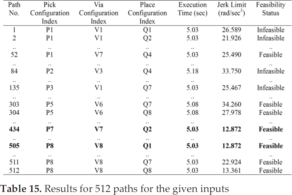
By considering all possible configurations at ‘V’, the resultant 512 (8×8×8) paths are generated by this algorithm connecting pick, via and place destinations. These paths are in turn evaluated for collision, as specified in section 3.5.7, and the feasible path(s) is/are identified. Table 15 provides the execution time, jerk and feasibility status of 512 paths generated by the algorithm.

Table 15.

Results for 512 paths for the given inputs

Path No.	Pick Configuration Index	Via Configuration Index	Place Configuration Index	Execution Time (sec)	Jerk Limit (rad/sec3)	Feasibility Status
1	P1	V1	Q1	5.03	26.589	Infeasible
2	P1	V1	Q2	5.03	21.926	Infeasible
..	..	..	..	..		..
52	P1	V7	Q4	5.03	25.490	Feasible
..	..	..	..	..		..
84	P2	V3	Q4	5.18	33.750	Infeasible
..	..	..	..	..		..
135	P3	V1	Q7	5.03	25.467	Infeasible
..	..	..	..	..		..
303	P5	V6	Q7	5.08	34.260	Feasible
..	..	..	..	..		..
304	P5	V6	Q8	5.08	27.978	Feasible
..	..	..	..	..		..
434	P7	V7	Q2	5.03	12.872	Feasible
..	..	..	..	..		..
505	P8	V8	Q1	5.03	12.872	Feasible
..	..	..	..	..		..
511	P8	V8	Q7	5.03	22.924	Feasible
512	P8	V8	Q8	5.03	13.361	Feasible

3.6.4 Selection of best feasible path and configurations

The least time-consuming path with minimum jerk is selected as the optimal path interpolating pick, via and place destinations. For the above-given input data, the minimum execution time is calculated as 5.03 seconds, which is achieved in 321 instances out of 512. The path number 434 with respective pick, via and place configurations P7, V7 and Q2, and the path number 505 with respective pick, via and place configurations P8, V8 and Q1, whose minimum jerk limit was 12.872 rad/sec³ and minimum path time 5.03 sec, are the best solutions for the given inputs. These paths show the lowest time and jerk values among all other feasible paths.

Figure 15 and Figure 16 depict the corresponding trajectories of displacement, velocity, acceleration, jerk and torque for the optimal solutions, i.e., trajectories for all the joints of the PUMA 560 robot during its motion along the paths 434 and 505, respectively.

Figure 15.

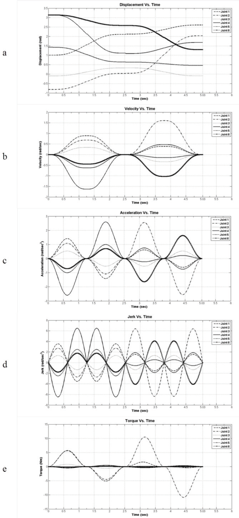
STST of PUMA 560 for one of the optimal solutions, i.e., path no. 434 among 512 paths: a) Displacement, b) Velocity, c) Acceleration, d) Jerk, e) Torque

Figure 16.

STST of PUMA 560 for one of the optimal solutions, i.e., path no. 505 of 512 paths: a) Displacement, b) Velocity, c) Acceleration, d) Jerk, e) Torque

When it fails to obtain a feasible path, the algorithm selects another via-point randomly from R(x_v,y_v,z_v) and identification of feasible paths will be carried out again. This procedure will be continued until a feasible path is obtained. The proposed algorithm has the difficulty of ensuring the optimal path; also, it is assumed that the orientation at via-point is the average of the orientation of destinations, which may not ensure the best configuration at via-point.

4. Results and Discussion

This section first discusses the performance of the proposed S-curve trajectory generated with the sine wave form of the jerk profile by comparing the cubic spline trajectory with the constant jerk profile presented by Chettibi et al. [1] for the weighted cost function, giving a relative importance to minimizing transfer time and joint efforts or power.

The results given in [1], with the various weighting coefficients of transfer time function μ and joint efforts α between 1 and 0, are used for the comparison. Table 16 compares the performance of the proposed algorithm with the results presented in [1]. It reveals that the proposed trajectory performs better than the cubic spline trajectory when joint efforts are given more weightage than the execution time. Hence, this S-curve trajectory can be implemented in applications where smoothness in object handling is of great significance, to ensure motion with less vibration.

Table 16.

Performance comparison of proposed STST

Secondly, the performance is tested for the situations that require a via-point to provide a collision-free trajectory. In order to check the influence of via-point on the optimality of the solution, six experiments, with the same input as used in stage two (trajectory with via-point) (section 3.0), are conducted with via-points selected around the obstacle. Table 17 shows the results.

Table 17.

Results of the experiments on the search algorithm for various via-points

Experiment No.	Location of the via point			Best Execution Time (sec)	Jerk Limit (rad/sec3)	Feasibility Status
	X	Y	z
1	−0.026	0.228	0.428	5.03	12.872	Feasible
2	0.394	−0.195	0.340	−-	−-	Infeasible
3	0.260	0.328	0.428	5.03	8.857	Feasible
4	0.260	0.328	0.734	5.03	10.498	Feasible
5	0.260	0.000	0.234	5.03	6.108	Feasible
6	−0.500	−0500	0.100	5.03	14.974	Feasible

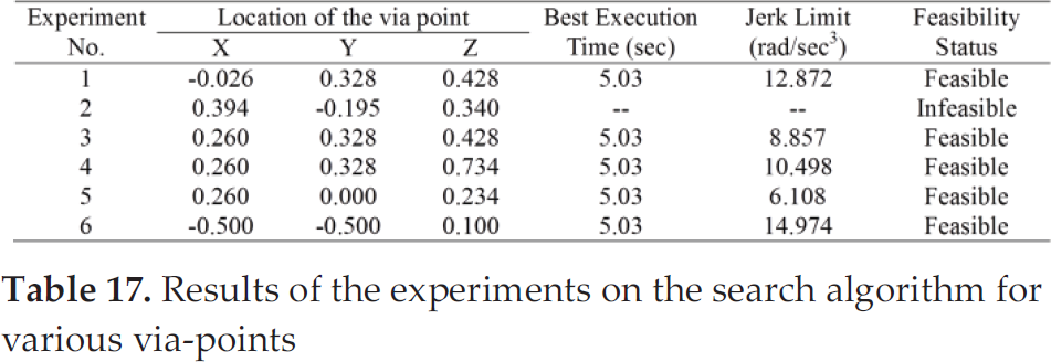
It can be observed that certain points lead to infeasible solutions and the jerk values for the optimal solution vary with via-point. It can also be seen that there are solutions with the same minimum execution time but they different minimum jerk value, based on the location of the via-point.

Although execution time is the same for the optimal solutions at various locations of via-point, a differentiation in the jerk values can also be observed in the results. A method is therefore required to identify the best via-point in the dexterous workspace for achieving the optimal solution with both the minimum jerk and time.

It can also be observed that the jerk, acceleration and velocity profiles are similar for alternate optimal solutions (Figure 15 and Figure 16) of the algorithm, although there will be changes in robot pose. With variations in the location of the via-point, the algorithm provides the better solution as illustrated and sometimes provides infeasible solutions as well.

5. Conclusion

An automated trajectory planner for near-optimal trajectory of 6-DOF robotic manipulators for the given Cartesian description of end-effector at pick and place destinations under kinematic constraints has been described in this work. Li et al.'s (2007) acceleration-bounded S-curve trajectory is modified as a jerk-bounded S-curve trajectory (i.e., all trajectories, displacement, velocity and acceleration, are generated within the specified maximum jerk value) so as to obtain a smoother movement without any abrupt changes. A mathematical model with the objective of minimum execution time for pick-and-place operations is formulated by including a ‘forbidden sphere’ technique to avoid obstacles and a jerk-bounded synchronized trigonometric S-curve trajectory to ensure smooth motion. A two-stage algorithm to find the optimal trajectory with or without via-point is proposed. The performance of the proposed trajectory planner is analysed through comparison with the results of [1]. This reveals that the proposed S-curve trajectory is smoother than the cubic spline trajectory. Also, the proposed STST provides better results when joint efforts are considered with higher priority than execution time. Further, the possibility to set maximum bounds for the jerk before executing the trajectory allows for a large stability and safety margin. Since the proposed algorithm ensures that the jerk of the resulting trajectory will be kept under the limit values set a priori by the user, the resulting vibrations will also be kept low. Hence, the S-curve trajectory is suitable for applications in which smoothness (low vibration) in object handling is of great significance. The proposed planner is able to handle the trajectory with and without via-point and traces the smooth, collision-free, near-time-optimal trajectory. The collision-free trajectory is ensured not only for the robot's end-effector but also for its links. The performance test carried out for the situations requiring a via-point to provide a collision-free trajectory indicates that the optimal solutions with different via-points are the same for minimum time, but differ in terms of jerk values. This requires searches with many via-points in the dexterous space for a smooth and minimum-time trajectory. A method for identifying suitable via-points to obtain the optimal solution quickly is therefore required. This work has also considered the enumeration technique to identify the minimal robot execution time with all possible configurations of pick, via and place destinations in the dexterous workspace – this is computationally difficult and huge amounts of data are involved. Future work will be devoted to extending this algorithm to find out the optimal via-point by means of suitable intelligent heuristics. This work has considered a single objective function, minimization of execution time which can be extended with more than one objective function, such as minimization of time and jerk and minimization of time and energy.