Sage Journals: Discover world-class research

Abstract

This article presents a non-collision trajectory planning algorithm in three-dimensional space based on velocity potential field for robotic manipulators, which can be applied to collision avoidance among serial industrial robots and obstacles, and path optimization in multi-robot collaborative operation. The algorithm is achieved by planning joint velocities of manipulators based on attractive, repulsive, and tangential velocity of velocity potential field. To avoid oscillating at goal point, a saturated function is suggested to the attractive velocity potential field that slows down to the goal progressively. In repulsive velocity potential field, a spring damping system is designed to eliminate the chattering phenomenon near obstacles. Moreover, a fuzzy logic approach is used to optimize the spring damping coefficients for different velocities of manipulators. Different from the usual tangential velocity perpendicular to the repulsive velocity vector for avoiding the local minima problem, an innovative tangential velocity potential field is introduced that is considering the relative position and moving direction of obstacles for minimum avoidance path in three-dimensional space. In addition, a path priority strategy of collision avoidance is taken into account for better performance and higher efficiency when multi-robots cooperation is scheduled. The improvements for local minima and oscillation are verified by simulations in MATLAB. The adaptabilities of the algorithm in different velocities and priority strategies are demonstrated by simulations of two ABB robots in Robot Studio. The method is further implemented in an experimental platform with a SCARA and an ABB robot cooperation around a stationary obstacle and a moving object, and the result shows real time and effectiveness of the algorithms.

Keywords

Robotic manipulators collision avoidance trajectory planning 3-D VPF path priority

Introduction

To meet the requirements of flexible and agile manufacture, multi-robot cooperation that enables the completion of tasks faster, cheaper, and more reliable is drawing more attention. However, the working environment as well as tasks for robots will be more complex and diverse. Therefore, it becomes particularly important in many applications for robots in avoiding collision with each other and other objects, such as cooperative assembly,¹ coordinated handling,² and remote monitoring.³

Currently, there are lots of studies on robots collision avoidance mainly with the following solution.

(1) A* algorithm

A* algorithm is one of the best known path planning algorithms, which can be applied on metric or topological configuration space. This algorithm uses a combination of heuristic searching and searching based on the shortest path. However, these results were not entirely satisfactory and good, and the computational time was very large.⁴ So some modifications of A* algorithm or accelerated search strategy are suggested.^4

–7

(2) Configuration space

The configuration space or C-space in robot path planning is defined as the set of all possible configurations of a robot. C-space is N-dimensional where N is the number of degrees of freedoms of the robot.⁸ Each point in it uniquely represents one position of the robot, for example, the position and orientation of a mobile robot or the joint angles of an industrial manipulator.⁹ This method is generally utilized to avoid stationary obstacles.¹⁰

(3) Grid modeling

Grid method uses grid to be units of environmental information during path planning, and environment is quantified as grid having a certain resolution. It can avoid the complex calculations when dealing with the boundaries of the obstacles.¹¹ This method can be applied to path planning in three-dimensional (3-D) environment.¹² The size of the grid has a direct impact on the length of the planning and precision, so it will also take up a lot of storage space if the working area is large and planning path is very accurate.¹³

(4) Probabilistic road maps (PRMs) and rapidly-exploring random trees (RRTs)

The most well-known sampling-based algorithms include PRM and RRT. However, PRMs tend to be inefficient when obstacle geometry is not known beforehand.¹⁴ RRTs have the advantage that they expand very fast and bias toward unexplored regions of the configuration space and so covering a wide area in a reduced time.¹⁵ Although the RRT algorithm quickly produces candidate feasible solutions, it tends to converge to a solution that is far from optimal.¹⁶

(5) Artificial potential field

In collision-free algorithms, the artificial potential field (APF) method firstly introduced by Khatib¹⁷ is particularly attractive due to its simplicity and efficiency. The basic concept of APF is that robot moves from a starting point to a goal point with the action of attractive potential function and repulses away from the obstacles with the action of repulsive potential function. The establishment of APF is simple and fast, which makes it popular for collision-free path planning of mobile robots and articulated manipulators.

For the original APF, robot under the action of virtual force moves from the starting point to the goal point without colliding with obstacles.^18

–21 So the method is also called force potential field (FPF).

However, Barbara²² presents that the FPF method based on the force or torque mode is difficult to carry out on practical industrial robot. Jaryani²³ proposes the concept of velocity potential field (VPF). Unlike the traditional force control approach, VPF transforms distances into the velocity of robot and has no concern of dynamic issues. The attractive velocity is assigned the vector of making the robot head toward an identified goal. In contrary to the attractive field, the repulsive velocity has inverse effect on the robot and it generates a differential motion vector that points the robot backward to the obstacle.

APF method may suffer from local minima problem when attractive and repulsive forces/velocities confront each other on the same line. Many solutions, such as using virtual target^24
–26 or introducing a tangential potential field,^19,27 have been put forward on it. To bypass obstacles, a tangential potential field is usually applied normal to the repulsive potential field.

VPF is a simple and direct method and is applied in collision-free trajectory planning of mobile robots, articulated robot manipulators, and unmanned aerial vehicle.

Kitts²⁸ defines the attractive velocity as a constant from the current point to the target point. The repulsive field includes a repulsive translational velocity and an angular velocity. The repulsive velocity magnitude may be a constant or changes in strength with an inverse proportion of the r-th power of distance between the robot and obstacle, where r is greater than or equal to one. The angular velocity component can solve the local minima problem. To make sure robots arrive at the target quickly, the attractive function usually sets a higher speed. When approaching the goal, the robot may pass the goal in the next periodic interval with the speed that may result in oscillation near the goal. Huang²⁹ defines that attractive velocity is proportional to the distance between the robot and the target. For the repulsive velocity, a radius of the influence of the repulsive field is suggested. Within the circle of influence, the magnitude of the vector grows from zero (outside or on the edge of the circle of influence) to a speed in inverse proportion to the distance between the robot and the obstacle. Jaryani²³ introduces a radius of influence of the attractive field, outside of this circle of extent, the vector magnitude keeps a constant and higher value. Within this circle of extent, the vector magnitude is set proportional to the distance between the robot and the goal. When the robot reaches the goal, the attractive velocity is reduced to zero. The repulsive potential has the same definition as in the study by Kitts et al.²⁹

The abovementioned studies are VPF-based collision avoidance happened in two-dimensional (2D) space.

Hu³⁰ proposes a method based on velocity vector field for unmanned aerial vehicle path planning. Actually, the path is planned in 2-D space for the projection of terrain. Attractive velocity function is defined as a constant speed. The repulsive velocity is inversely proportional to the square of the distance between planning points and threat points. The tangential velocity has the same value as the repulsive velocity, whose direction is perpendicular to the repulsive velocity pointing to the side of the target point. OuYang and Zhang³¹ have a study on collision avoidance with industrial manipulators. Attractive velocity function is defined as a constant speed. An approaching velocity of the manipulator and the obstacle is introduced for repulsive velocity function (RVF). The repulsive velocity is active when the distance between the manipulator and the obstacle falls within the circle of influence and the approaching velocity is less than zero, which indicates the manipulator is approaching the obstacle. The smaller the distance and/or the approaching velocity is, the higher the repulsive velocity is. A detour velocity is deployed to escape local minimal here. The vector of detour velocity is calculated by the vector cross-product without the consideration of obstacle relative position to the robot or moving direction. Wu³² studies the method to grasp a static or moving object with collision avoidance in dynamic environments. Attractive vector contains the translation and rotation information to approach the target. The translation part has a linear relationship with the distance between the end-effector and the target, the rotation part relates to the rotation of the target. Repulsive vector magnitude is evaluated using the exponential of robot–obstacle distances, and the direction relies on all obstacle points. According to the final attractive vector and repulsive vector, the local minima escaping strategy is determined to apply or not. The potential vector is generated by attractive and repulsive vectors that are different in various cases.

In this article, a more applicable algorithm is proposed based on VPF in 3-D working space of robot collaboration around obstacles. Based on the form in the study by Jaryani,²³ VPF is improved by introducing a saturation function at attractive VPF and designing a fuzzy spring damping system in repulsive VPF for a more smooth and time-efficient trajectory. Furthermore, an innovative tangential VPF is proposed for minimum avoidance path in 3-D space that is considering more factors, such as the current position relations of obstacles, target, and robots, and moving direction of the obstacle. In addition, a path priority strategy of collision avoidance is introduced for better performance and higher efficiency when multi-robots cooperation is scheduled.

The architecture of robots collaboration with collision avoidance is shown in Figure 1.

Figure 1.

Architecture of robots collaboration with collision avoidance.

The geometry and parameters of robots are built offline. Joint angles of robots are retrieved from their encoders. The location and geometry of obstacles are known here by a binocular vision system that was introduced in the study by Huang.³³ All these information are shared in local area network (LAN) in real time.³⁴ Based on a simplified model of robots and obstacles, the nearest distance is estimated among robots and obstacles. Then a set of joint velocities is generated by collision-free algorithms and the robot motion control commands are sent to the controller to operate the manipulators, which are updated at a specified time interval until the manipulator reaches the goal.

The article is organized as follows: The “Simplified model and distance estimating” section describes the simplified models of objects by swept sphere volumes (SSVs) and the estimation of the minimum distance. An improved collision avoidance algorithm based on VPF is presented in the “An improved collision-free algorithm based on VPF” section. The “Simulations and experimentation” section expounds the implementation of simulation and experiments and the “Conclusions” section devotes to the conclusions.

Simplified model and distance estimating

The effectiveness of the proposed algorithm largely depends on the method of estimate of distance between objects. Using SSV bounding box technology that can be applied to construct a hierarchical tree and approach the object geometry gradually to represent complex objects, the minimum distance detection can be performed more efficiently and accurately.

Swept sphere volumes

If Q denotes swept path, S denotes primitive, then the collection of points can be formed by S swept Q as follows

sweep (S, Q) = \cup S_{c}

where S_c denotes S at location c. Q has three geometric primitives which are points, line segments, and rectangles.

The swept spheres formed by primitives are point swept spheres (PSSs), line segments swept spheres (LSSs), and rectangle swept spheres (RSSs). As a result, the geometric model of the manipulator can be simplified by a list of SSVs.

Hierarchies of simplified model

According to the characteristics of manipulators, a method of two-layer hierarchies of simplified model is proposed as follows:

Step 1: Layer one

As shown in Figure 2(a), the manipulator is only represented by a RSS.

Figure 2.

The simplified model of robot. (a) Layer one. (b) Layer two.

Step 2: Layer two

Layer two will be checked when the potential collision is not eliminated in layer one. In this layer, the manipulator is represented by mixed SSVs, as shown in Figure 2(b).

Distance checking

As shown in Figure 3, there are two SSVs (two LSSs in Figure 3(a), one LSS and one RSS in Figure 3(b) in the space. C_i and C_j are SSVs, L_i and L_j are geometric primitives, r_i and r_j are the radius of L_i and L_j, respectively. The approximate distance between the two SSVs is

d_{i j} = d (L_{i}, L_{j}) - r_{i} - r_{j}

where $d (L_{i}, L_{j})$ is the distance between the primitives L_i and L_j, which can be obtained through space analytic geometry.³⁵

Figure 3.

Distance estimate of SSVs. SSVs: swept sphere volumes. (a) LSS to LSS. (b) LSS to RSS.

Assuming object #p is represented by m_p SSVs and they are ${{}^{p}C_{1}, {}^{p}C_{2} \dots {}^{p}C_{m_{p}}}$ , object #q is represented by m_q SSVs and they are ${{}^{p}C_{1}, {}^{p}C_{2} \dots {}^{p}C_{m_{q}}}$ . Then the matrix of distance checking is

d_{m_{p} \times m_{q}}^{pq} = [\begin{matrix} d_{11}^{p q} & \dots & d_{1 j}^{p q} & \dots & d_{1 m_{q}}^{p q} \\ ⋮ & ⋮ \\ d_{i 1}^{p q} & \dots & d_{i j}^{p q} & \dots & d_{i m_{q}}^{p q} \\ ⋮ & ⋮ \\ d_{m_{p} 1}^{p q} & \dots & d_{m_{p} j}^{p q} & \dots & d_{m_{p} m_{q}}^{p q} \end{matrix}]

where $d_{i j}^{p q}$ is the distance of SSV ${}^{p}C_{i}$ and ${}^{q}C_{j}$ , $i = 1, 2 \dots m_{p}, j = 1, 2 \dots m_{q}$ .

The minimum distance $d_{0}^{p q}$ between object #p and object #q is

d_{0}^{p q} = min {d_{i j}^{p q}}

An improved collision-free algorithm based on VPF

VPFs in 3-D space

VPFs are defined in 3-D workspace of manipulators as shown in Figure 4. Attractive velocity function (AVF) $\vec{v_{a}}$ ensures end-effector $N (x, y, z)$ head toward goal point $G (x_{G}, y_{G}, z_{G})$ , whose speed is associated with the distance between N and G and the direction is from N to G.

Figure 4.

The velocity potential fields. (a) Static obstacle. (b) Moving obstacle.

RVF $\vec{v_{r}}$ is formed around obstacles for avoiding collision when the robot approaches the obstacle to a certain distance, which is claimed as a radius of repulsive potential field d_r, the smaller the distance is, the greater the repulsive velocity is, $R (x_{R}, y_{R}, z_{R})$ and $O (x_{o}, y_{o}, z_{o})$ are the nearest two points between the robot and the obstacle, and then the direction of $\vec{v_{r}}$ is from O to R.

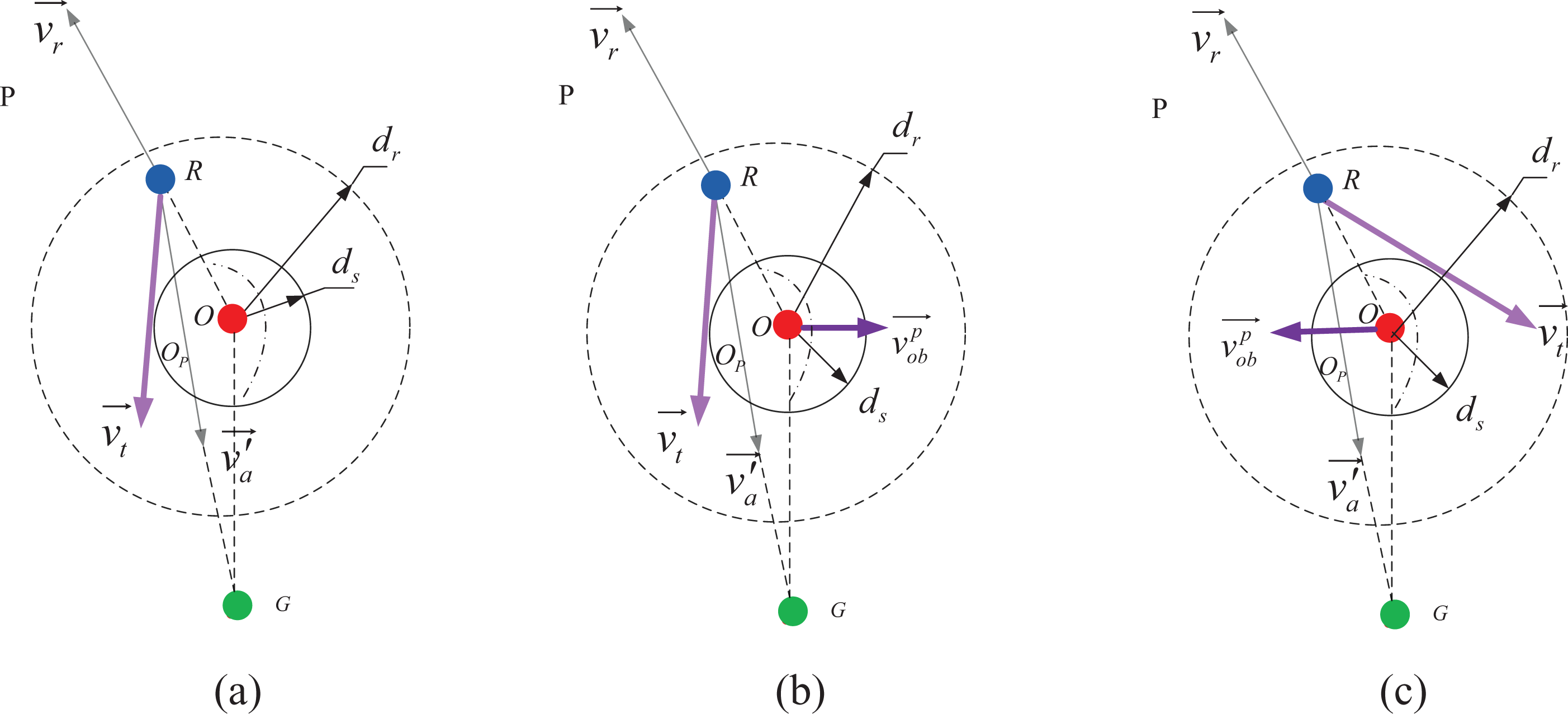
A safe area of sphere O with a radius d_s is set. O_P is a circle-shaped cross section of the sphere O in the plane P that is formed by $\vec{v_{r}}$ and $\vec{{v^{'}}_{a}}$ as shown in Figure 5. $\vec{{v^{'}}_{a}}$ is the equivalent speed at point R to $\vec{v_{a}}$ at point N. Tangential velocity function (TVF) $\vec{v_{t}}$ is used to bypass obstacles to avoid the local minima problem. To make sure the path of collision avoidance in 3-D space as short as possible, $\vec{v_{t}}$ should be tangent to the circle O_P. η is an angle from OR clockwise rotation to OG in the plane P.

Figure 5.

Tangential velocity field. (a) Static obstacle. (b) Moving obstacle: $\vec{v_{o b}^{p}}$ inside of η. (c) Moving obstacle: $\vec{v_{o b}^{p}}$ outside of η.

For stationary obstacle, if η > 180°, the direction of $\vec{v_{t}}$ is tangent to the circle O_P in the opposite side of η as shown in Figure 5(a). If η < 180°, $\vec{v_{t}}$ is in the side of η. If η = 180°, $\vec{v_{t}}$ can be either side of η. For moving obstacle, the direction of moving obstacle should be considered and $\vec{v_{o b}^{p}}$ is the component of the obstacle velocity in the plane P. If the direction of $\vec{v_{o b}^{p}}$ falls within the angle η, to avoid possible collision of robot and dynamic obstacles, then the direction of $\vec{v_{t}}$ can be on the opposite side of η as shown in Figure 5(b). Otherwise the direction of $\vec{v_{t}}$ is on the side of η as shown in Figure 5(c).

AVF with saturation function

When approaching the goal, the robot may pass the goal in the next periodic interval with a large velocity. Therefore, a saturation function is suggested to AVF to reduce the chattering as the robot gets closer to the goal. Assume that there is a boundary layer of radius d_a around the goal. Attractive velocity is defined as a constant outside of the boundary layer, and the distance between the robot and the goal decreases in the boundary layer. Hence, the attractive velocity v_a is defined as

v_{a} = {\begin{cases} K ‖ \vec{N G} ‖ > d_{a} \\ K \cdot ‖ \vec{N G} ‖ / d_{a} ‖ \vec{N G} ‖ \leq d_{a} \end{cases}

where K is the strength of the attractive velocity potential function and it is a constant that can be set to maximum possible value. $‖ \vec{N G} ‖$ is the distance between N and G.

Now, the AVF is defined as

\vec{v_{a}} = v_{a} \frac{\vec{N G}}{‖ \vec{N G} ‖}

where $\vec{N G} = {(x_{G} - x, y_{G} - y, z_{G} - z)}^{T}$ .

For robotic manipulator operating in 3-D space, the reference vector is related to location and orientation of the end-effector in operational space. Therefore, both linear velocity and angular velocity need to be controlled.

According to the manipulator end-effector orientation based on job task, the angular velocity of the robot is defined as

\vec{ω_{a}} = [\begin{array}{l} ω_{x} \\ ω_{y} \\ ω_{z} \end{array}] = [\begin{matrix} sin θ \cdot sin ψ & cos ψ & 0 \\ sin θ \cdot cos ψ & - sin ψ & 0 \\ cos θ & 0 & 1 \end{matrix}] [\begin{array}{l} \dot{φ} \\ \dot{θ} \\ \dot{ψ} \end{array}]

where $\dot{φ} = \frac{v_{a} \cdot (φ_{G} - φ)}{‖ \vec{N G} ‖}$ , $\dot{θ} = \frac{v_{a} \cdot (θ_{G} - θ)}{‖ \vec{N G} ‖}$ , $\dot{ψ} = \frac{v_{a} \cdot (ψ_{G} - ψ)}{‖ \vec{N G} ‖}$ ; φ, θ, and ψ are the robot’s Euler angles and φ_G, θ_G, ψ_G are the robot’s final Euler angles.

In most cases, the Jacobian matrix is not a square matrix when translating velocity in Cartesian space into velocity in joint space. Therefore, pseudoinverse Jacobian matrix piv(J) needs to be constructed, which is defined as

piv (J) = {(J^{T} \cdot J)}^{- 1} \cdot J^{T}

Using the inverse Jacobian relationship, we will have the joint velocities

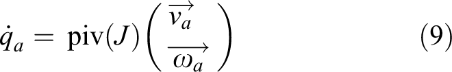
{\dot{q}}_{a} = piv (J) (\begin{array}{l} \vec{v_{a}} \\ \vec{ω_{a}} \end{array})

where J is Jacobian matrix, $J = (\vec{J_{1}}, \dots, \vec{J_{i}}, \dots, \vec{J_{n}})$ and n is the number of robot joints.

RVF based on fuzzy spring damping system

As the same reason of the oscillation near the goal, the trajectory of the robot at the edge of RVF will be rough. In order to make the robot have a smooth trajectory when it repels the edge of repulsive VPF, a virtual spring damping system is introduced into RVF, whose coefficients are k_p and k_d around an obstacle as shown in Figure 6; the system generates a repulsive velocity v_r when robot enters into the repulsive potential field. No matter the robot entering or leaving repulsive potential field, the damping system will “dissipate” the robot’s energy (velocity). Affected by damping, the oscillation of the robot will be reduced near the obstacle.

Figure 6.

Virtual spring damping system.

Based on the spring damping system, the repulsive velocity v_r, within the distance of influence d_r, is defined as

v_{r} = k_{p} \cdot (d_{r} - d_{0}) + k_{d} \cdot (d_{r} - d_{0})^{'}

where d₀ is the closest distance between the robot and the obstacle $d_{0} = ‖ \vec{O R} ‖ = \sqrt{{(x_{R} - x_{O})}^{2} + {(y_{R} - y_{O})}^{2} + {(z_{R} - z_{O})}^{2}}$ , and $(d_{r} - d_{0})^{'}$ is the first derivative of $(d_{r} - d_{0})$ .

The coefficient $k_{p} (k_{d}) \geq 0$ is positively correlated to the velocity v. Generally, the velocity of manipulators varies in different stages or tasks. In order to make the algorithm have a better self-adaptability to different velocities of manipulators, an optimization of k_p and k_d by fuzzy logic approach is implemented.

The velocity v of a manipulator moving toward an obstacle is chosen as input and $k_{p} (k_{d})$ is defined as output. v is divided into five fuzzy sets: Very Slow (VS), Slow (SL), Medium (M), Fast (FA), and Very Fast (VF). v’s membership function diagram is shown in Figure 7.

Figure 7.

v’s membership function.

$k_{p} (k_{d})$ is divided into five fuzzy sets: Very Small (VSL), Small (SM), Medium (ME), Big (BG), and Very Big (VB). According to simulation results and experimental experiences, the membership functions of k_p and k_d are shown in Figure 8 and Figure 9, respectively.

Figure 8.

k_p's membership function.

Figure 9.

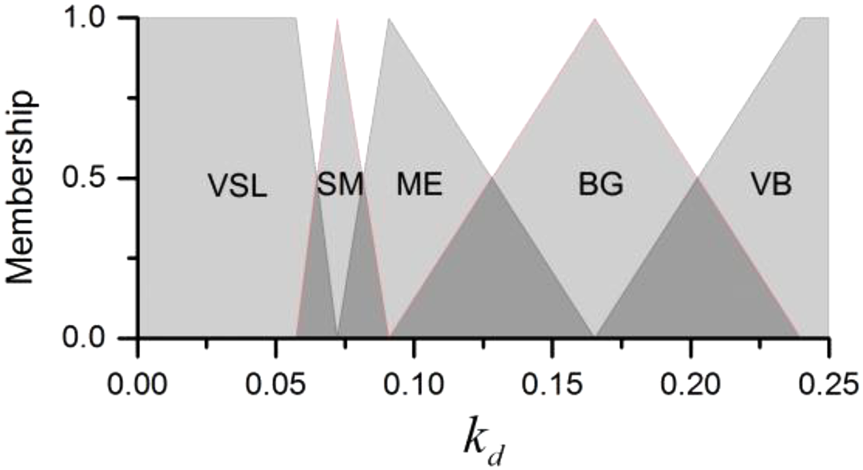
k_d's membership function.

The following fuzzy control rules shown in Table 1 are designed.

Table 1.

Fuzzy control rules.

IF	v	VS	SL	M	FA	VF
THEN	$k_{p} (k_{d})$	VSL	SM	ME	BG	VB

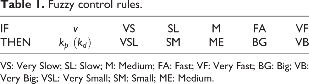
VS: Very Slow; SL: Slow; M: Medium; FA: Fast; VF: Very Fast; BG: Big; VB: Very Big; VSL: Very Small; SM: Small; ME: Medium.

Then RVF can be expressed as follows

\vec{v_{r}} = {\begin{cases} M \cdot \frac{\vec{OR}}{‖ \vec{OR} ‖} d_{0} \leq d_{s} \\ v_{r} \cdot \frac{\vec{OR}}{‖ \vec{OR} ‖} d_{s} < d_{0} \leq d_{r} \\ {(0, 0, 0)}^{T} d_{0} > d_{r} \end{cases}

where M denotes a large positive number $\vec{OR} = {(x_{R} - x_{O}, y_{R} - y_{O}, z_{R} - z_{O})}^{T}$ .

The repulsive velocity is zero outside of influence of repulsive potential field. Within the influence, the velocity is determined by the spring damping system. If a manipulator and an obstacle are very close, the repulsive velocity would be infinite.

In order to get joint velocities, partial Jacobian matrix J′ is created. Point R is assumed that locates on the joint m as the end-effectors of the manipulator, so only the effects of joints between R and the robot base are considered.³⁶ Then J′ is defined as

J^{'} = (\vec{J_{1}}, \cdot \cdot \cdot, \vec{J_{i}}, \cdot \cdot \cdot \vec{J_{m}}, \vec{O})

where $\vec{O} = {[\begin{matrix} 0 & \dots & 0 \\ ⋮ & ⋱ & ⋮ \\ 0 & \dots & 0 \end{matrix}]}_{6 \times (n - m)}$ .

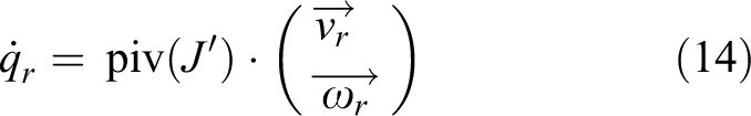
Thus joint velocities can be expressed by “partial Jacobian matrix” relationship for $\vec{v_{r}}$ as

(\begin{array}{l} \vec{v_{r}} \\ \vec{ω_{r}} \end{array}) = J^{'} \cdot {\dot{q}}_{r}

where $\vec{ω_{r}} = (0, 0, 0)^{T}$ denotes the angular velocity of manipulator.

Then joint velocities ${\dot{q}}_{r}$ are expressed as

{\dot{q}}_{r} = piv (J^{'}) \cdot (\begin{array}{l} \vec{v_{r}} \\ \vec{ω_{r}} \end{array})

Tangential velocity function

TVF is defined as

\vec{v_{t}} = {\begin{cases} M \vec{p} d_{0} \leq d_{s} \\ γ (d_{r} - d_{0}) \vec{p} d_{s} < d_{0} \leq d_{r} \\ {(0, 0, 0)}^{T} d_{0} > d_{r} \end{cases}

where $\vec{p}$ is unit directional vector of tangential VPF that has been defined in the “VPFs in 3-D space” section. γ is the strength of the potential field obtained by fuzzy logic approach in the same way as $k_{p} (k_{d})$ . Figure 10 shows the membership functions of γ.

Figure 10.

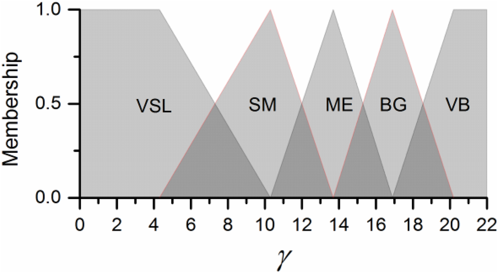
γ’s membership function.

Similarly, ${\dot{q}}_{t}$ can be expressed as

{\dot{q}}_{t} = piv(J^{’}) \cdot (\begin{array}{l} \vec{v_{t}} \\ \vec{ω_{t}} \end{array})

where $\vec{ω_{t}} = {(0, 0, 0)}^{T}$ .

Real-time collision avoidance with path priority strategy

Different from one manipulator avoiding an obstacle, robots can avoid each other for multiple robots. For this issue in the study by OuYang F and Zhang,³¹ all robots are seen as moving obstacles. The manipulators apply 0.6 times of the repulsive velocity when all the repulsive velocity needs to be added up in two robots’ avoidance collision.

Actually, different priorities should be considered in path planning of multiple robots for process optimization or synergetic work. For example, if two robots are requested to arrive at a place for collaboration, the best choice is to let the robot with longer distance have the shorter path with little waiting time and the other robot should give way to avoid collisions with each other, so the robot with longer distance should have higher priority and the other behave as “subordinates.”

Therefore, a variable α ( $α \in [0, 1]$ ) is introduced for robot priority level, α = 0 is the highest priority, α = 1 is the lowest priority, and there is $\sum_{j = 1}^{m_{r}} α_{j} = 1$ for m_r robots’ cooperation. The higher the priority of the robot is given, the smaller its repulsive velocity and tangential velocity are, then the shorter its avoidance path is.

For m_o obstacles and m_r robots in the workspace, according to equations (9), (14), and (16), the velocity vector of the kth(1 ≤ k ≤ m_r) robot joint space that added priority factor is defined as

{\dot{q}}^{k} = {\dot{q}}_{a}^{k} + \sum_{i = 1}^{m_{o}} ({\dot{q}}_{r}^{i} + {\dot{q}}_{t}^{i}) + α_{k} (\sum_{j = 1, j \neq k}^{m_{r}} ({\dot{q}}_{r}^{j} + {\dot{q}}_{t}^{j}))

where ${\dot{q}}_{r}^{i}$ ( ${\dot{q}}_{r}^{j}$ )和 ${\dot{q}}_{t}^{i}$ ( ${\dot{q}}_{t}^{j}$ ) are repulsive joint velocities and tangential joint velocities generated by the ith obstacle and the jth robot, respectively.

In addition, joint angle limits and joint velocity limits existed in all actual manipulators should be taken into account.

The output of the algorithm is a set of joint velocities that command the robot to move during the following time interval. However, some manipulators are position controlled and in this case the joint velocities can be converted into joint positions at the end of each time interval, that is

q_{l} (t + Δ t) = q_{l} (t) + {\dot{q}}_{l} (t) \cdot Δ t

where q_l(t) is the position of joint l at time t, Δt is the time interval.

If the robot is in a singular position ( $| J (q) | = 0$ ), the Jacobian matrix cannot be reversed. In this case, the method of “singular separation + damping reciprocal” cited in the study by Peng³⁷ is used to achieve singular avoidance.

Simulations and experimentation

The simulation environment and experimental setup are constructed to demonstrate the capability and effectiveness of the proposed method. The simulations are conducted in MATLAB and Robot Studio (developed by ABB) environment, respectively. The experimental setup consists of two manipulators, one robot is ABB (IRB120) and the other is SCARA (developed by Googol). The control software is written in Microsoft Visual Studio.

Simulations in MATLAB

AVF with saturation function

In this simulation, a comparison of the proposed AVF in the article with other two algorithms is implemented, and the result is shown in Figure 11. AVF1 is derived from the studies by Kitts et al.,²⁸ Hu and Li,³⁰ and OuYang and Zhang³¹ that keeps with a fixed speed to a goal. AVF2 from the studies by Huang²⁹ and Wu³² will decrease as the distance between the robot and the target with a directly proportional relationship.

Figure 11.

Performance of the different AVFs. AVFs: attractive velocity functions.

The robot begins to move toward the target at the same speed. When approaching the goal with AVF1, the robot moves backward and forward again and again, which makes the robot oscillate near the goal. AVF2 and the proposed function make the robot smoothly get closer and closer to the target. Compared with AVF2, the robot reaches the goals faster in the proposed velocity because the robot begins to slow down near the goal.

RVF based on fuzzy spring damping system

In this simulation, the robot moves from starting point A (100, 380) to goal point B (400, 0), while a static obstacle of radius 30 mm is located at O (200,200). d_r is 50 mm. A comparison of different RVFs with robot speed of 10 and 50 mm/s is shown in Figure 12(a) and (b), respectively.

Figure 12.

Trajectories with different RVFs. (a) Robot with a speed of 10 mm/s. (b) Robot with a speed of 50 mm/s. RVFs: repulsive velocity functions.

Repulsive velocities in the literature^23,28
–30 are related to $d_{0}^{- r}$ $(r \geq 0)$ , and RVF1, RVF2, and RVF3 correspond to r = 0, r = 1, and r = 2, respectively. RVF4 from the study by Wu³² changes with $exp(- d_{0})$ .

As shown in Figure 12, the trajectories of robot are oscillating near the obstacle at different levels when applied in the RVF1, RVF2, RVF3, and RVF4, although the oscillation can be improved as the robot speed increases for the RVF3. For the proposed function in this article, the trajectories of the robot keep the shortest and smoothest path while avoiding the obstacle whether the robot speed is low or high.

TVF with different directions

In this simulation, an obstacle of cylinder with 50 mm radius and 100 mm height is located at O (200, 200, 0). Plane L is perpendicular to $\vec{v_{r}}$ in 3-D space. As shown in Figure 13, $\vec{v_{0}}$ , $\vec{v_{1}}$ , $\vec{v_{2}}$ , $\vec{v_{3}}$ , and $\vec{v_{4}}$ in the plane L are examples of tangential velocity which is perpendicular to $\vec{v_{r}}$ as usual, and $\vec{v_{t}}$ is the defined tangential velocity in this article.

Figure 13.

TVF with different directions.

The robot moves from point S (0, 400, 0) to point G (400, 0, 100). The simulation results are shown in Figure 14 that the path of the robot keeps the shortest by applying $\vec{v_{t}}$ . Compared to all other tangential velocity in the plane L, $\vec{v_{0}}$ lies the smallest angle with $\vec{{v^{'}}_{a}}$ , so the robot with $\vec{v_{0}}$ has the second shortest path after $\vec{v_{t}}$ .

Figure 14.

Trajectories with different TVFs. (a) 3-D map. (b) Top view. TVFs: tangential velocity functions. 3-D: three-dimensional.

Simulations in Robot Studio

Collision avoidance in different velocity

This simulation is carried out in Robot Studio with two ABB robots, $α_{1} = α_{2} = 0.5$ . Point (330, −180, 520) and (320, 210, 590) are the starting point and goal point of robot #1 and point (370, 180, 520), (370, 180, 520) are for robot #2, d_r = 50 mm.

The simulation results are indicated in Figures 15 to 17. As shown in Figure 15, the distance between the two robots always keeps positive which means the collision never occurs. The collision avoidance processes between the two robots are shown in Figure 16 (v = 50 mm/s). At around t = 2 s, the robots enter repulsive potential field and begin to mutual repulsion. At approximately t = 5 s, the robots leave repulsive potential field and move to their own goals. Figure 17 presents the smooth trajectories of the robot joints.

Figure 15.

Time diagram of the distance between the two robots.

Figure 16.

Collision avoidance processes (down: front view, up: top view). (a) t = 0 s. (b) t = 2 s. (c) t = 2.5 s. (d) t = 3 s. (e) t = 3.8 s. (f) t = 5 s. (g) t = 6 s. (h) t = 9 s.

Figure 17.

Time-joint angle curve of robot #1.

Path priority strategies in process of collision avoidance

In this simulation, there are five priority levels for robot #1 and robot #2 in which $(α_{1}, α_{2})$ are (0, 1), (0.25, 0.75), (0.5, 0.5), (0.75, 0.25), and (1, 0), respectively. Starting point and goal point are the same as those in simulation in the “Collision avoidance in different velocity” section.

The trajectories of end-effectors of robot #1 and robot #2 are shown in Figure 18. If robot #1 is required to arrive at the goal as quickly as possible, it would be given the highest priority (α₁ = 0) which means robot #1 has the shortest path from the starting point to the goal point. In order to avoid collisions, robot #2 behaves as a “subordinate” robot (α₂= 1) and thoroughly gives way to robot #1. If robot #1 owns higher priority than robot #2 at a level of α₁ = 0.25 and α₂ = 0.75, the paths of two robots are plotted in the yellow line where robot #1 has shorter path. And vice versa while the robot #2 has the highest or higher priority level as in purple or green lines. The magenta line represents the paths of the two robots with identical priority.

Figure 18.

Trajectories of the two robots with different priorities.

Experiment

In this experiment, robot ABB (IRB120) and SCARA working in an overlapped working envelope are set up. The collision avoidance algorithm is implemented on two robots with two obstacles of which one is stationary and the other is moving. The base coordinate of SCARA is defined as global coordinate frame. ABB robot moves from A(480, 240, 200) to B(380, −240, 200) at a speed of 10 mm/s. Starting point and goal point of SCARA are C(100, 400, 100) and D(400, 0, 100) with a speed of 25 mm/s. Static obstacle represented by a LSS (radius: 40, length: 180) is located at (200, 180, 50). An object staying on a moving belt at a speed of 20 mm/s which is represented by a LSS (radius: 70, length: 200) can be considered as a dynamic obstacle. In this scenario, SCARA and ABB robot have the same priority level.

Figure 19 records the behaviors of collision avoidance in different time intervals. The trajectories of the two robots and a moving obstacle at the projection of XY plane are shown in Figure 20, which are denoted in the same color at the same time. Figure 19(a) is in the initial state. Figure 19(b) shows the two robots are moving toward their own goal without obstacles. Figure 19(c) and (d) shows the process of SCARA avoiding the static obstacle and ABB robot avoiding the dynamic obstacle, which correspond to ① and ② in Figure 20(a). When t = 25 s as shown in Figure 19(e), SCARA robot almost arrives to the goal D and ABB robot prepares to avoid SCARA. Figure 19(f) and (g) show that the two robots are avoiding collision with each other, which correspond to ③ in Figure 20(a). As shown in Figure 19(h), the two robots are succeeded in reaching their own goals without any collisions. From Figure 20(b), which magnifies the trajectories in Figure 20(a), it can be found that the trajectories are very smooth when the robots enter or leave repulsive potential field. Experiment results show the two robots successfully avoid collision with each other and the two obstacles.

Figure 19.

Collision avoidance process among robots and obstacles. (a) t = 0. (b) t = 5 s. (c) t = 10 s. (d) t = 20 s. (e) t = 25 s. (f) t = 30 s. (g) t = 35 s. (h) t = 46 s.

Figure 20.

Trajectories of robots and moving obstacle. (a) Trajectories at the projection of XY plane. (b) Magnification of trajectories near obstacles.

Conclusions

In this article, a real-time algorithm based on VPF is introduced to coordinate collision-free trajectories for robotic manipulators in 3-D space. The robot velocity is modeled by AVF, RVF, and TVF, which plan an optimal collision-free trajectory. Compared with the applications of the current methods based on VPF, the AVF with a saturation function makes the robot reach the goal faster without oscillation, the RVF with a fuzzy spring damping system has enhanced the optimum trajectories as well as the adaptability to different velocities while avoiding the obstacle. A new method of TVF is created to get the shortest path in 3-D space, considering the moving direction of the obstacle and the relative positions of obstacles, target, and robots currently. The control algorithm of multi-robots cooperation takes robot priority strategies into avoiding collision among robots that makes it more flexible in path planning and gets more coordinating paths based on the task importance and the time spent of every robot working.

The desired outcomes of the algorithms are verified in the simulations, which not only solve the problems of local minima around obstacle and oscillation near the obstacle and goal but also show better performances in trajectory or path planning. An experiment of the two robots working around a stationary obstacle and a moving obstacle is executed, and the results illustrate the effectiveness of the proposed method in real-time collision avoidance among robots and stationary or moving obstacles. Future works on this algorithm include optimizing the collision path further in consideration of moving obstacle velocity magnitude, and investigating its feasibility in narrow channels.

Footnotes

Declaration of conflicting interests

The author(s) declared no potential conflicts of interest with respect to the research, authorship, and/or publication of this article.

Funding

The author(s) disclosed receipt of the following financial support for the research, authorship, and/or publication of this article: This work has been supported by the Science and Technology Planning Projects of Guangdong Province (2014B090920001).

ORCID iD

JM Zhai

References

Kinugawa

Kawaai

Tanaka

. Collision risk reduction system for assembly task partner robot. In: 2012 IEEE/ASME international conference on advanced intelligent mechatronics, Kaohsiung, Taiwan, 11–14 July 2012, pp. 280–285. IEEE.

Wangmanaopituk

Voos

Kongprawechnone

. Collaborative nonlinear model-predictive collision avoidance and path following of mobile robots. In: ICROS-SICE international joint conference 2009, Fukuoka, Japan, 18–21 August 2009, pp. 3205–3210.

Zhang

Yuan

. An automatic collision avoidance approach for remote control of redundant manipulator. In: 2008 IEEE international conference on information and automation, Zhangjiajie, Hunan, China, 20–23 June 2008, pp. 809–814. IEEE.

Duchon

Babinec

Kajan

. Path planning with modified a star algorithm for a mobile robot. Model Mech Mechatron Syst 2014; 96: 59–69.

Zidane

Ibrahim

. Wavefront and a-star algorithms for mobile robot path planning. In: 2017 3rd international conference on advanced intelligent systems and informatics, Cairo, Egypt, 9–11 September 2017, pp. 69–80. IEEE.

Zhai

Liu

. An efficient approach for collision-free trajectory planning using adaptive velocity vector field algorithm. In: 2017 international conference of mechanical design and the 19th annual conference on mechanical design, Beijing, China, 19–21 December 2017, pp. 1169–1190. IEEE.

Wang

. Indoor mobile-robot path planning based on an improved A* algorithm. Press Tsinghua Univ 2012; 52: 1085–1089.

Verwer

BJH

. A multiresolution work space, multiresolution configuration space approach to solve the path planning problem. In: Proceedings of the 1990 IEEE international conference on robotics and automation, Cincinnati, OH, USA, 13–18 May 1990, pp. 2107–2112. IEEE.

Ademovic

Lacevic

. Path planning for robotic manipulators via bubbles of free configuration space: evolutionary approach. In: 2014 22nd Mediterranean conference on control and automation, Palermo, Italy, 16–19 June 2014, pp. 1323–1328. IEEE.

10.

Ademovic

Lacevic

. Path planning for robotic manipulators using expanded bubbles of free C-space. In: 2016 IEEE international conference on robotics and automation, Stockholm, Sweden, 16–21 May 2016, pp. 77–82. IEEE.

11.

Wang

Chen

. Path planning algorithm of level set based on grid modeling. In: 2010 international conference on computer design and applications, Qinhuangdao, Hebei, China, 25–27 June 2010, pp. V5508–V5510. IEEE.

12.

Zhang

. An algorithm for mobile robot path planning based on a 3D grid map. J Xian Jiaotong Univ 2013; 47: 57–61.

13.

Wang

Kai

. Path planning for robot based on grid algorithm. Agri Equip Vehicle Eng 2009; 4: 14–17.

14.

Qureshi

Ayaz

. Intelligent bidirectional rapidly-exploring random trees for optimal motion planning in complex cluttered environments. Robot Auto Syst 2015; 68: 1–11.

15.

Jorge

Slawinski

Mut

. Online path planning based on rapidly-exploring random trees. In: IEEE-ICIT 2010 international conference on industrial technology, Vina del Mar, Chile, 14–17 March 2010, pp. 1451–1456. IEEE.

16.

Sertac

. Anytime Motion Planning using the RRT. In: 2011 IEEE international conference on robotics and automation, Shanghai, China, 9–13 May 2011, pp. 1478–1483. IEEE.

17.

Khatib

. Real-time obstacle avoidance for manipulators and mobile robots. Int J Robot Res 1986; 5(1): 90–98.

18.

Ding

. Vision trajectory planning for mobile robots based on hybrid artificial potential field. J Zhejiang Univ Sci B 2016; 50: 1298–1306.

19.

Masoud

. Decentralized self-organizing potential field-based control for individually motivated mobile agents in a cluttered environment: a vector-harmonic potential field approach. IEEE Trans Syst Man Cybern A Sys Hum 2007; 37: 372–390.

20.

Xing

. A new method for robot path planning based artificial potential field. In: 2016 11th IEEE conference on industrial electronics and applications, Hefei, China, 5–7 June 2016, pp. 1294–1299. IEEE.

21.

Wang

Lyu

Yao

. Three-dimensional path planning for unmanned aerial vehicle based on interfered fluid dynamical system. Chin J Aero 2015; 28(1): 229–239.

22.

Barbara

. A framework for implementing cooperative motion on industrial controllers. IEEE Trans Robot Auto 2004; 20(3): 583–589.

23.

Jaryani

. An effective manipulator trajectory planning with obstacles using virtual potential field method. In: 2007 IEEE international conference on systems, man, and cybernetics, Montreal, QC, Canada, 7–10 October 2007, pp. 1573–1578. IEEE.

24.

Yamashita

Asama

. An efficient improved artificial potential field based regression search method for robot path planning. In: 2012 IEEE international conference on mechatronics and automation, Chengdu, China, 5–8 August 2012, pp. 1227–1232. IEEE.

25.

Zheng

Wilfrid

. Real-time local path planning for mobile robots. In: 2013 9th international workshop on robot motion and control, Wasowo, Poland, 3–5 July 2013, pp. 215–220. IEEE.

26.

Zou

Jing

. Virtual local target method for avoiding local minimum in potential field based robot navigation. J Zhejiang Univ Sci B 2003; 4(3): 264–269.

27.

Masoud

. Constrained motion control using vector potential fields. IEEE Trans Syst Man Cybern Syst A Sys Hum 2000; 30: 251–272.

28.

Kitts

Stanhouse

Cindaphorm

. Cluster space collision avoidance for mobile two-robot systems. In: 2009 IEEE/RSJ international conference on intelligent robots and systems, St. Louis, MO, USA, 11–15 October 2009, pp. 1941–1948. IEEE.

29.

Huang

. Velocity planning for a mobile robot to track a moving target—a potential field approach. Robot Auto Syst 2009; 57(1): 55–63.

30.

. Application in real-time planning of UAV based on velocity vector field. In: International conference on electrical and control engineering, Wuhan, China, 26–28 June 2010, pp. 5022–5026. IEEE.

31.

OuYang

Zhang

. Virtual velocity vector-based offline collision-free path planning of industrial robotic manipulator. Int J Adv Robo Syst 2015; 12(9): 129.

32.

. Grasping the object with collision avoidance of wheeled mobile manipulator in dynamic environments. In: 2013 26th IEEE/RSJ international conference on intelligent robots and systems, Tokyo, Japan, 3–8 November 2013, pp. 5300–5305. IEEE.

33.

Huang

. Research on the working environment 3D information detection of the industrial robot based on binocular vision. Thesis, South China University of Technology, Guangzhou, China, 2017.

34.

Zhai

Lianzhong

Peisen

GUO

. Design and experiment on M2M2A of multi-robot intelligent collaboration. Robot 2017; 39(4): 415–422.

35.

Chen

Liang

. Detection collision algorithm for two-manipulator system. J Beijing Univ Aero Astro 2013; 39: 1644–1648.

36.

Bosscher

Daniel

. Real-time collision avoidance algorithm for robotic manipulators. In: 2009 IEEE international conference on technologies for practical robot applications, Woburn, MA, United states, 9–10 November 2009, pp. 113–122. IEEE.

37.

Peng

. Singular avoidance and vibration suppression in trajectory planning of 6-DOF serial robot. Thesis. Harbin Institute of Technology, China, 2015.

A novel non-collision trajectory planning algorithm based on velocity potential field for robotic manipulator

Abstract

Keywords

Introduction

Simplified model and distance estimating

Swept sphere volumes

Hierarchies of simplified model

Distance checking

An improved collision-free algorithm based on VPF

VPFs in 3-D space

AVF with saturation function

RVF based on fuzzy spring damping system

Tangential velocity function

Real-time collision avoidance with path priority strategy

Simulations and experimentation

Simulations in MATLAB

AVF with saturation function

RVF based on fuzzy spring damping system

TVF with different directions

Simulations in Robot Studio

Collision avoidance in different velocity

Path priority strategies in process of collision avoidance

Experiment

Conclusions

Footnotes

Declaration of conflicting interests

Funding

ORCID iD

References