
Abstract
A voltage-based control scheme for robot manipulators has been presented in recent literature, where feedback linearization is applied in the electrical equations of the DC motors in order to cancel the electrical current terms. However, in this paper we show that this control technique generates a system of the form Ex = Ax + Bu, where E is a singular matrix, that is to say, a generalized state-space system or singular system. This paper introduces a formal stability analysis of the respective system by considering the state-space equation as a singular system. Furthermore, in order to avoid the singularity of the closed-loop system, modified voltage-based control schemes are proposed, whose Lyapunov stability analyses conclude semiglobal asymptotic stability for the set-point control case and uniform boundedness of the solutions and semiglobal convergence of the position, as well as velocity errors for the tracking control case. The proposed control systems are simulated for the tracking and set-point cases using the CICESE Pelican robot driven by DC motors.
1. Introduction
Many control techniques have been proposed to solve the motion control problem of robot manipulators. One of the most commonly used techniques has been the torque-based control. Many design techniques for torque-based controllers can be found in the literature (robust control [1], adaptive control [2], intelligent control [3]). Nevertheless, the above torque-based control schemes neglect the inner current loops of the actuator drivers and suppose that the torque control action, required by the controller, is supplied directly to the actuator inputs.
Other control strategies can be found in the literature (velocity-based control [4], voltage-based control [5], passivity-based control [6], etc.). In [5], a voltage-based control for robots manipulators with DC motors is presented. A feedback linearization is applied on the electrical model equation of the DC motor to cancel the electrical current terms. However, this operation requires that the voltage-based control has a state-feedback and, even more, a derivative state-feedback (non-proper control law [7] presenting undesirable impulsive responses). The approach of generalized systems is a tool which is able to describe derivative actions in non-proper systems. Some techniques to approximate a non-proper stabilizing control law for a proper system [7], [8] exist. In this paper, by using generalized systems theory, a formal stability analysis for the voltage-based control in robot manipulators presented in [5] is introduced. Some alternative voltage-based controllers which can be described by proper systems are presented whose Lyapunov stability analyses are also introduced. As a consequence of the analysis for the set-point (or regulation) problem, two variants of the voltage-based controller are presented. The previous proposed schemes are also generalized for the case of the tracking control problem. The proposed control systems are simulated for regulation and tracking control using the CICESE Pelican robot [9] which is driven by permanent magnet DC motors.
The paper is organized as follows. In Section 2, the control law presented in [5] is analysed and an alternative voltage-based control is proposed. A stability analysis for the proposed voltage-based controller is presented in Section 3 and a second variant is introduced. The generalization to the tracking control case is also presented in this section. Simulation results for each of the proposed controllers are presented in Section 4 and finally some conclusions are given in Section 5.
2. Voltage-Based Control
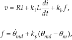
The electrical model of a permanent magnet DC motor is described by the following equation:
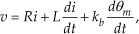
where R is the armature resistance, L is the armature inductance, kb is the back emf constant, v is the armature voltage, i is the armature current and θ m is the rotor position, respectively.
We can rewrite (1) as

The dynamic model of the permanent magnet DC motor is given by

where T is the load torque, τm is the motor torque, r is the gear reduction coefficient, Jm is the sum of actuator and gear inertia, and Bm is the damping coefficient. The motor torque τm is proportional to the armature current as

where km is the torque coefficient. For the permanent magnet DC motor, the torque coefficient is equal to the back emf constant, this is

By using (1), (3) and (4), we obtain the following open-loop system

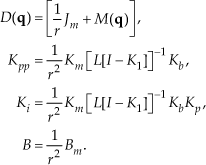
Now, we can use the following control law which is presented in [5]:

where θ md is the desired rotor position, θ md is the desired rotor velocity and kp>0 is a constant gain. By substituting control law (7) into (1), and by using (3) and (4), we can obtain the following closed-loop system
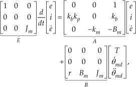
where

Since E is a singular matrix (due to the exact cancellation of the term
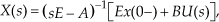
where x(0-) are the initial conditions of the states for t = 0-(an instant before t = 0). The behaviour of this kind of system is considerably different compared with the case when E is non-singular, as we show in the following:
The number of independent values that Ex(0-) can take, is reduced.
The transfer function G(s) may no longer be strictly proper; it may be written as the sum of a strictly proper part G(s) and a polynomial part D(s).
The free response of the system (u(t) = 0) exhibits, in addition to exponential motions, impulsive motions.
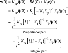
The free response of the system (8), using (10), is the following [10]:

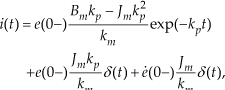
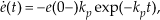
where δ(t) is the impulsive function. We can note from (12) that i(t) has an undesirable impulsive response. This impulsive response is due to the step that results from the initial condition ė(0-) (given by the initial state of the system an instant before the closed-loop system begins to work) falling to ė(0) calculated from (13) in t = 0 (ė(0) = -e(0-)kp) [10].
Indeed, the impulsive response only could be theoretically avoided if the equation

is fulfilled, because the use of (14) in (12) cancels the impulsive terms. From the previous reasoning and taking into account that
In order to get a practical synthesis of control law (7) for cancelling the singularity of the system (8), we propose the following control law, which is a slight but important improvement on (7)
where k 1 < 1 is a constant. For the case when k 1 = 1, we obtain the voltage-based control presented in [5].
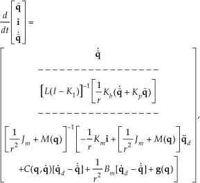
With the objective of working with n-link serial rigid robots, we will consider n permanent magnet dc motors, which drive each joint of the manipulator. To this end, by applying control law (15) for each actuator in the robot manipulator, and using (1), (3) and (4), we obtain the following closed-loop system

where
The main feature of the closed-loop system (16) is that it becomes in a non-singular system which does not present impulsive responses and it can be analysed by the classical Lyapunov stability techniques.
Now, we consider a serial n-link rigid robot, whose dynamics can be written as

where
Let us consider that the load torque T in (16) is given by the robot dynamics (17), that is

By substituting (18) into (16), we have the following closed-loop system
where we have used

to write the closed-loop system in terms of the joint position error vector
3. Stability Analysis
With the purpose of making the stability analysis easy it is convenient to consider the following change of variables

The closed-loop system (19) can be expressed in function of the new variables as follows:
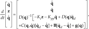
where
3.1 Set point control
For the case of set point control problem, we have that q̇ d =0 and q̈ d =0. Then, we can rewrite (15) as

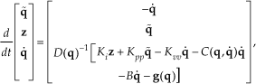
and, based on (22), we can obtain the following closed-loop system

whose equilibrium point is

The closed-loop system (24) can be seen as a serial rigid robot (17) with a torque PID controller

where Kpp is the proportional gain matrix, B is the derivative gain matrix and Ki is the integral gain matrix. It is possible to prove that closed-loop system (24) is semiglobally asymptotically stable [9][11][12].
From (26) it can be seen that in the initial position the integral part cancels the proportional part. In order to avoid the robot keeping still at the beginning or avoid it beginning to move slowly, the integral gain must be sufficiently large [13][14]. However, according to [12], high derivative gains in control law (25) must also be selected in order to guarantee asymptotic stability. Nevertheless, note that the derivative gains matrix B is fixed and this cannot be changed. The above-mentioned is difficult to guarantee when the damping coefficient Bm is small.
A possible solution for changing the derivative gain B in the closed-loop system (24) is to add the term

By using the controller (27) instead of (15), and making the corresponding change of variables, we obtain
where now, unlike (24), it is possible to change the derivative gain Kvv, where

One might think that the use of the control law could be counterproductive in the sense that the joint acceleration
3.2 Tracking control
For the case of the tracking control problem, we have the case that the closed-loop system (22) has no any equilibrium point. However, it is possible to prove that the solutions of (22) are uniformly bounded [15], moreover,

where
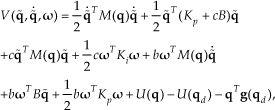
where c and b are constant parameters suitably chosen.
As it can be seen in [13], the system response is improved with high PI gains; this is achieved in the voltage-based controller (15) by setting the gains K1 close to 1. This makes control law (15) close to control 1 i aw (7).
Again, because we have used control law (15), we encounter the problem of not being able to vary the derivative gain. According to [16], with derivative gains relatively small, it is required that the trajectory be smooth, that is that the desired velocity q̇ d has a small value. In order to solve the above-mentioned problem, we propose the following control law:

which leads to the following closed-loop system:

The stability analysis of the closed-loop system (33) can be carried out in the same way as (22).
4. Simulations results
In this section we present simulation results using the voltage-based controllers (15), (32), (23) and (27) applied in a robot manipulator. We use the CICESE Pelican robot [9] of two degrees of freedom which, we have considered, is equipped with the brushed DC motors model MT-4060 ALYBE (joint 1) and MT-4060 BLYBE (joint 2) [17] whose parameters are presented in Table 1.
Numerical values of the parameters for the MT-4060 ALYBE and MT-4060 BLYBE DC motors

The simulations have been performed in Simulink (MatLab R2011a).
4.1 Tracking control simulation
Consider the desired trajectory presented in Figure 1 where the control objective is to move each joint from an initial position to a final position using a transient state trajectory as described in the following equation:

Desired trajectory for Simulation 1

where To is the initial time,
In this simulation control law (15) is used with

for both joints
The tracking errors are in the range of 1.5 × 10⁻⁶ [rad], as shown in Figure 2. The motor voltage and motor current are as shown in Figures 3 and 4, respectively. They are located under the valid limits values.

Tracking error of joints for control law (15)

Voltage of motors for control law (15)

Current of motors for control law (15)
It should be noted that, with the intention to emulate more closely control law (7) presented in [5], the gain k1 was also chosen closer to 1 (for example, k1 = 0.9995, k1 =0.9999, etc.); however, infinity problems in the numerical simulations were obtained.

Desired trajectory for Simulation 2
Because, by using control law (15) it is not possible to obtain small position errors and simultaneously to ensure that the motor voltage and the motor current are located under the valid limit values presenting little oscillations, control law (32) has been chosen to confront the above requirements in this simulation.
For this simulation control law (32) is now used with

for both joints.
As can be seen in Figure 6, the tracking errors do not exceed 9×10⁻⁴ [rad]. In Figures 7 and 8 the motor voltage and motor current are shown, respectively; they remain under the maximum permitted parameters.

Tracking error of joints for control law (32)

Voltage of motors for control law (32)

Current of motors for control law (32)
Once more, when the gain k1 is chosen closer to 1 in order to emulate control law (7) (for example, k1 = 0.9995, k1 =0.9999, etc.), simulation responses going to infinity are obtained.
Once again, we have considered control law (32) with the following gains:

for both joints.
The desired trajectories are approximately reached in 3 [s] for both joints, as can be seen in Figures 9, 10 and 11. By observing the above-mentioned figures, it is evident that the desired trajectory used in Simulation 1 with initial conditions of the position errors different to zero can easily be followed by using control law (32).

Joint position and desired position for joint 1

Joint position and desired position for joint 2
Tracking error of the joints for Simulation 3
The motor current and the motor voltage are shown in Figures 12 and 13. Despite the large current peak for joint 2, the electrical current and the voltage remain under the permitted maximum values.

Current of motors for Simulation 3
Voltage of motors for Simulation 3
4.2 Regulation control simulation
The controller gains chosen for control law (23) are:

for both joints.
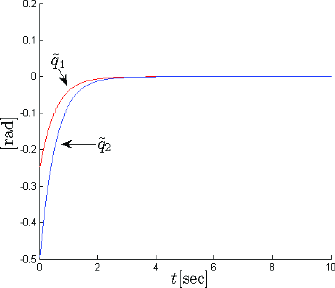
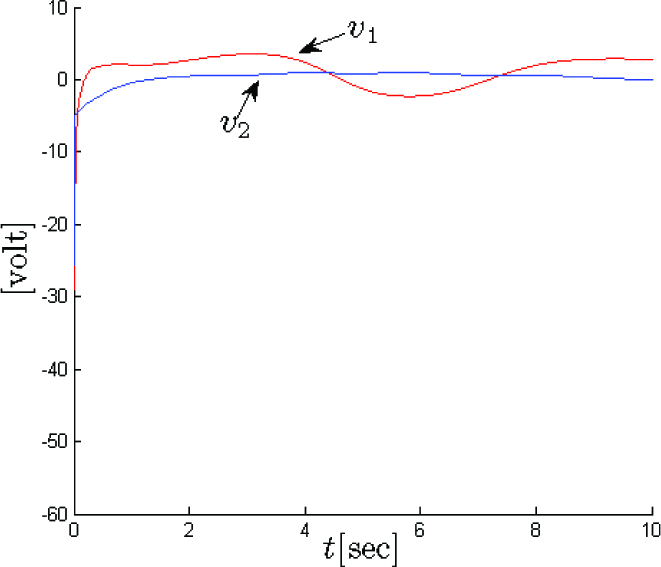
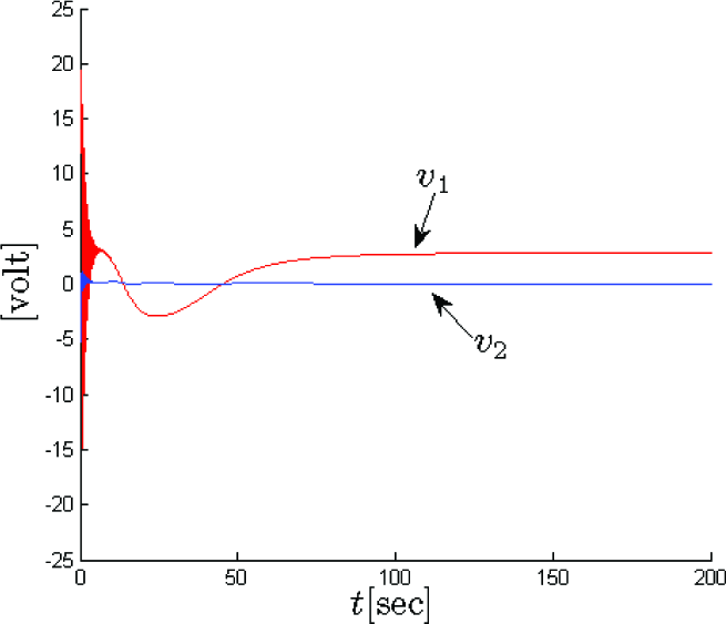
The desired positions are approximately reached in 140 [s] by the two joints (see Figure 14). The motor voltages and motor currents are shown in Figures 15 and 16, respectively. They are located under the valid limit values. However, as can be seen in Figure 17, the motor current responses are oscillating to a high degree and therefore, it is far from being acceptable in practical applications.

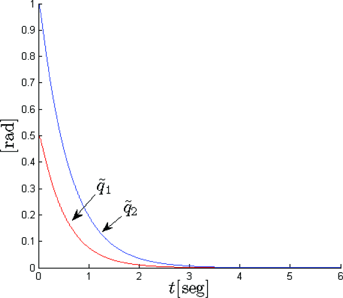
Joint position errors for control law (23)
Voltage of motors for control law (23)
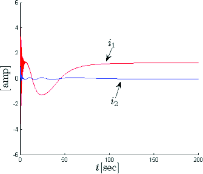
Current of motors for control law (23)

Currents of motors for control law (23) (zoom to 7 sec).
The controller gains chosen for control law (27) are

As can be seen in Figure 18, the desired joint positions are reached in 3 seconds for both joints. The motor currents and motor voltages are presented in Figures 19 and 20. It can be noted that the motor current responses have no oscillations. Note that the motor current i1 has an overcurrent peak of 15 [A]; however, this remains within the permitted technical specification.
Joint position errors for control law (27)

Voltage of motors for control law (27)

Current of motors for control law (27)
In order to ensure that the positions reach the desired set-points in less time than those shown in Figure 18, it might be required to protect the devices against damage due to overvoltage and/or overcurrent peaks caused by high gains, for example, by using saturated controls [18].
5. Conclusions
The voltage-based control presented in [5] for robot manipulators with DC motors has been analysed in this paper. This controller cancels the electrical current terms in the electrical model equation by using a feedback linearization. Toward this end, such a controller uses state and state derivative feedback. However, with this control law, a singular system is obtained which cannot be described by a classical state description. Therefore, by using the generalized systems theory, it has been shown in this paper that the electrical current responses have undesirable impulsive behaviours. In order to avoid such responses, two variants of the controller presented in [5] have been introduced, and moreover, the generalization to the tracking control case has been carried out. With these controllers, non-singular closed-loop systems are obtained and they have been analysed by using the classical Lyapunov theory. For the case of regulation control, semiglobal asymptotic stability is assured. In the tracking control case, it has been possible to prove that the solutions are uniformly bounded and
Footnotes
6. Acknowledgements
This work is partially supported by DGEST and CONACyT projects 134534 and 176587.