Sage Journals: Discover world-class research

Abstract

The article deals with the issue of using the Two Degree of Freedom (2DOF) PID controller to control an integral system and investigates by the simulation and experimental measurement what influence it has on the course of the control process compared to standard PID controller. The controlled plant is represented by the DC electric motor with worm gear and its output shaft rotation angle. The article studies the effect of the added parameters of the 2DOF controller on the dynamics of the closed-loop control. The influence of these parameters is then evaluated using the quality of feedback control criteria ITAE. The paper studies how the overshoot of the controlled variable during the setpoint step is eliminated using 2DOF control theory. The overshoot is caused due to an aggressive tuning of the controller to eliminate the disturbance effect on the controlled variable of the integral plants with dead zones.

Keywords

integral system 2DOF PID controller control system DC motor

Introduction

In the industrial environment today, the position control of various devices is a crucial task. We are increasingly encountering requirements to improve the accuracy and efficiency of production processes, where it is necessary to replace the positioning to the limit switches with feedback control to achieve optimal conditions for the technology. This task thus very often leads to integral system control, often with nonlinear properties, as described in the paper.¹

The typical approach for the feedback control is using the PD controller.^2–4 There is no permanent control deviation for linear integral systems such as pneumatic, electric, or hydraulic systems unless there are non-linearities like static friction. PID control can lead to removing the permanent control deviation in such systems.^5–7 However, the PID control may not always be ideal for this task, leading to overshoots and unwanted slip and slide effects. Therefore, it is often beneficial to use other algorithms that can handle the problem better. One such option is to use the PID controller algorithm with two degrees of freedom (2DOF).^8–13

Two Degree of Freedom PID controllers add setpoint weights for the proportional and derivative term of the algorithm to ensure that the effect of the disturbance is quickly eliminated while suppressing overshoot when tracking the setpoint.^8,9

The degree of freedom of a controller is defined as the number of closed-loop transfer functions that can be tuned independently,^14–18 which provides additional options for tuning the controller regarding change of setpoint or disturbance value.

Active disturbance rejection control, which uses the extended state observer^19–21 or the Disturbance observer,^22,23 can be used as an alternative. For both of these methods, we are required to create the inverse model of the plant. The simplification of the 2DOF controller is that the filter is applied to the setpoint signal and depends on already known PID parameters only. Due to that, the implementation of the 2DOF is also possible without the need for detailed knowledge about the plant. 2DOF controller can be tuned manually or by quantitative methods as^9,24 based on reducing the criteria described in Chapter 6. of this paper. Another option is also the combination of the 2DOF controller with the disturbance observer.²⁵ The same technique can also be used with other types of feedback loop control as Fuzzy control, which offer us the option to design the response properties based on expert experience, State controller, which allow us to design the control system based on the full state feedback, or Fractional PID control where the derivation and integration terms of PID controller are exchanged with the fractional-order integration and derivation term which leads to tackle the problem of dead zones nonlinearities in integral systems.²⁶ For both methods, the additional filter can be added to alternate the setpoint signal. However, the quantitative design of the filter for non-PID control is then based on Meta-heuristic optimization algorithms.²⁷ The implementation of the 2DOF filter was published before in ref. 28, where traditional 2DOF is modified to 2DOF with an internal model for time-delay processes. The combination of the 2DOF and Fractional PID controller design was then published in ref. 29. In the scope of this paper, we will focus on the traditional 2DOF PID Controller, where the design, implementation, and comparison between the numerical simulations and actual single-chip computer implementation.

Description of the system

The integral system (see Figure 1) is a DC motor with a worm gear, where the controlled variable is the angle of rotation of the output shaft. A resistance sensor provides the measurement in a potentiometric setup. The Arduino Nano microcontroller was used as a model control system to cooperate with an external AD converter and an adapting electronic board.

Figure 1.

DC motor as integral plant.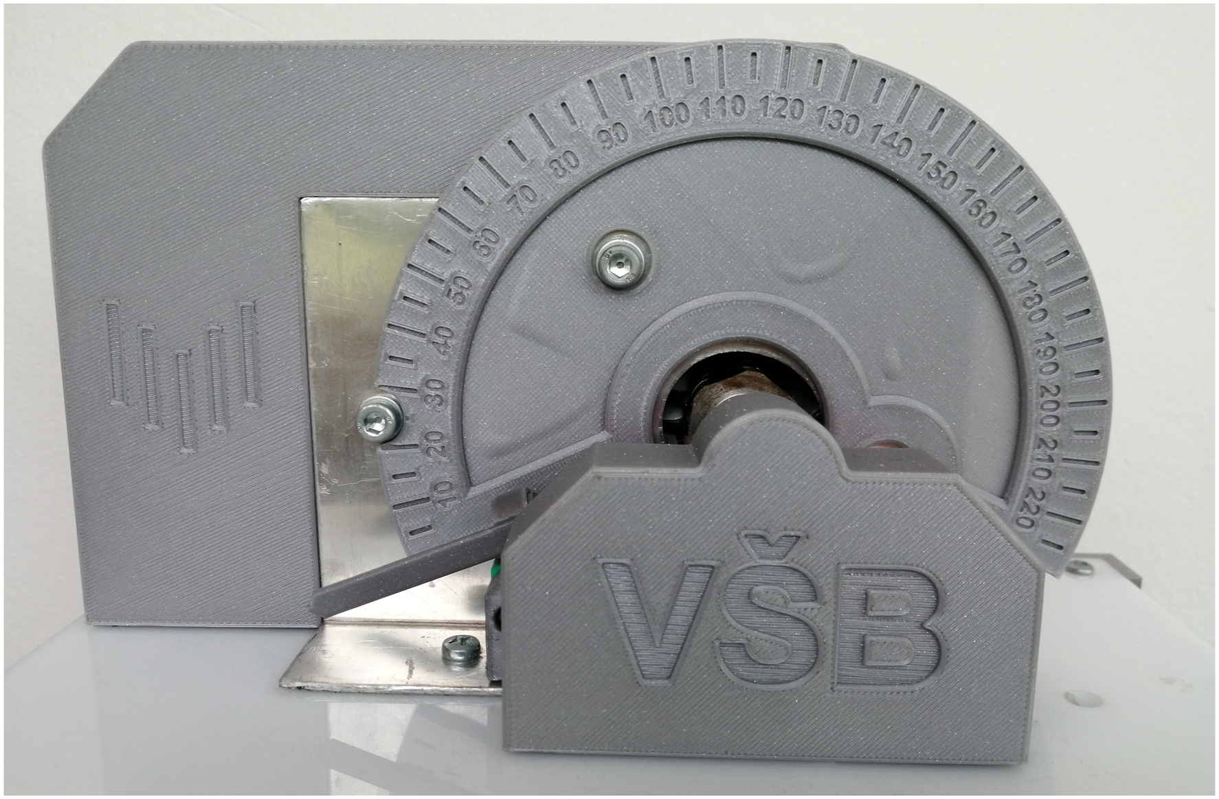

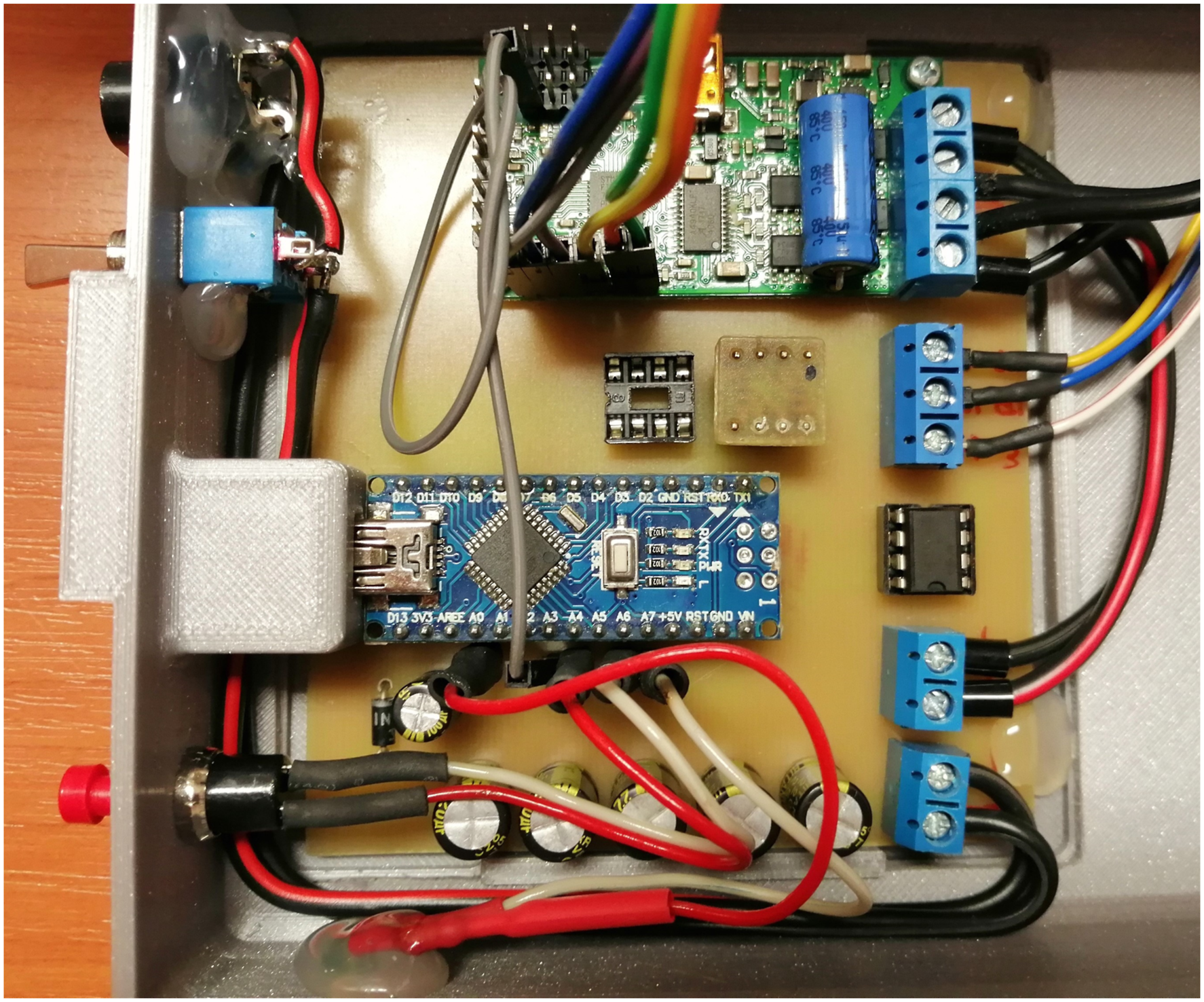
The action variable is realized via a DC motor driver (Pololu Simple High-Power Motor Controller 18v15, see Figure 2 and Figure 3) using a PWM signal and H-bridge direction switching as a response to the controller output. The MOSFET switching carrier frequency of the driver is 25 kHz. All the parameters of the driver are configurable through the USB port and dedicated software.

Figure 2.

Block diagram of the control system.

Figure 3.

Picture of the control system.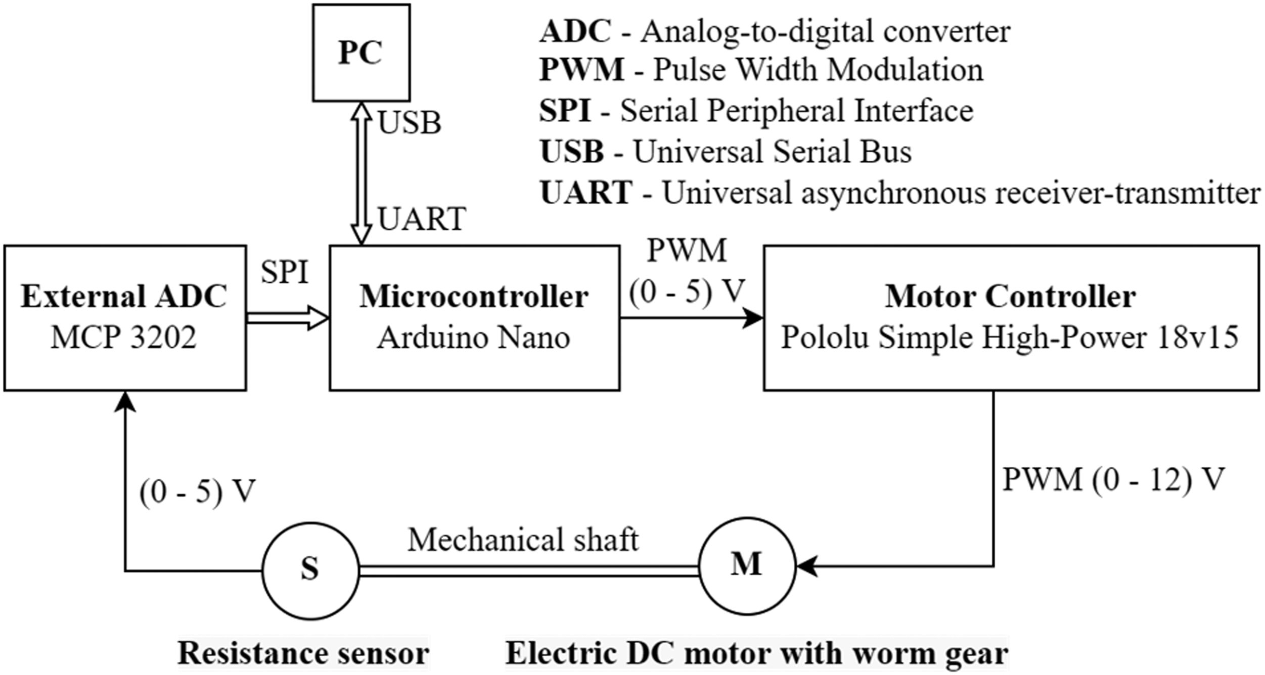

The output signal is an analog value in the range of 0–5 V processed by a 12-bit AD converter. The range of the angle of rotation of the output shaft is approximately 0–230°.

By its physical nature, the system itself exhibits nonlinearities, some of which are compensated by the algorithm, such as the initial insensitivity of the motor to the input signal caused by friction and nonlinear excitation of the motor coils. This behavior is relatively suppressed by the offset of the input signal to previously experimentally measured values. Other nonlinearities of the system were neglected for this work and considered in the identification of the system by selecting the most suitable system parameters.

Arduino nano was chosen as a suitable microcontroller-based control system to control this plant. Its main advantages are the possibility of fast and simple programming, easy portability of code to other similar boards, the possibility of programming from the MATLAB/Simulink environment while maintaining a low-cost concept, and easy implementation into existing hardware, unlike e.g., general PIC MCU.³⁰

The described block diagram of the control system can be seen in Figure 2. Figure 3 shows the electronics implementation of the experiment.

Theory of the 2DOF PID controller

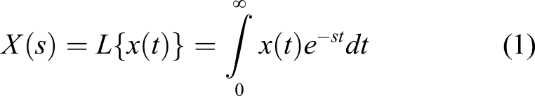
Our control system aims to calculate the correct control signal to the input of the plant described above. For the control, we are going to use the linear feedback controller. All the signals will be presented in the complex domain using the Laplace transform, whose definition is:

X (s) = L {x (t)} = \int_{0}^{\infty} x (t) e^{- s t} d t

(1)

Where the time (t) domain signal x(t) is transferred into the complex (s) domain X(s).

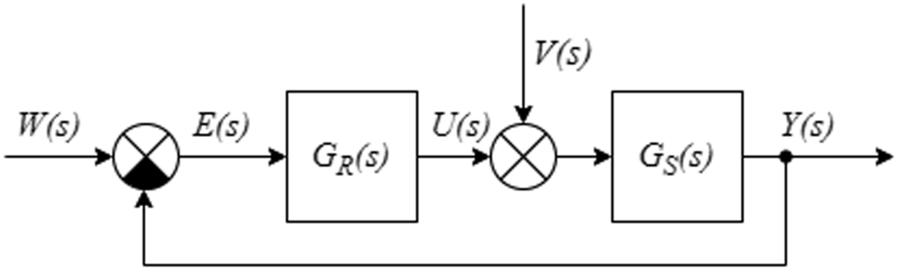
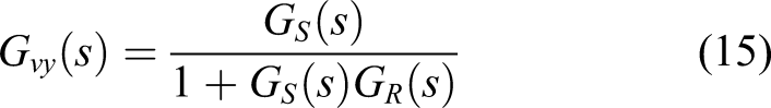
The primary method for controlling the plant state Y(s) is the Proportional-Integral-Derivative (PID) (based on Proportional, Integral, and Derivative terms) controller. The control loop diagram can be seen in Figure 4. This method uses the feedback from the control signal Y(s), which is then compared with the wanted (setpoint) signal W(s). The error signal can be calculated as:

E (s) = W (s) - Y (s)

(2)

Figure 4.

Closed loop control system diagram.⁹

Using the controller described by the transfer function:

G_{R} (s) = \frac{U (s)}{E (s)}

(3)

where U(s) is the control action signal which is the input to the controlled plant. The control plant transfer function describes the dynamics of the plant:

G_{S} (s) = \frac{Y (s)}{U (s)} | \begin{matrix} V (s) = 0 \end{matrix} = \frac{Y (s)}{V (s)} | \begin{matrix} U (s) = 0 \end{matrix}

(4)

where the V(s) is the disturbance.

Usually, during the design phase of the controller design, we set the expectation for the closed control loop to be:

The transfer function of the setpoint to the output is equal to one.

G_{w y} (s) = \frac{Y (s)}{W (s)} | \begin{matrix} V (s) = 0 \end{matrix} \to 1

(5)

The transfer function of the disturbance to the output is zero.

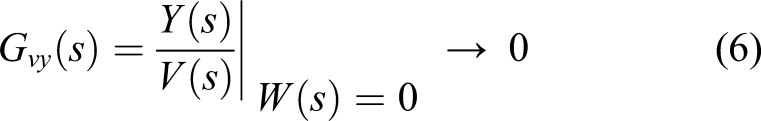
G_{v y} (s) = \frac{Y (s)}{V (s)} | \begin{matrix} W (s) = 0 \end{matrix} \to 0

(6)

Due to the physical property of the mechanical system, this expectation cannot be implemented as every state contain some dynamics, and the system cannot create the corresponding control signal against the future unknown disturbance V(s).

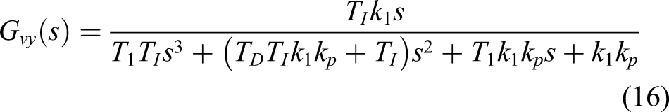
The difference between the standard PID controller and 2DOF PID controller will be presented on the plant, which was described above, and the experimental identification (described in the next chapter) lead to the transfer function:

G_{s} (s) = \frac{k_{1}}{s (T_{1} s + 1)}

(7)

where k₁ is the plant gain, and T₁ is the time constant due to inertia.

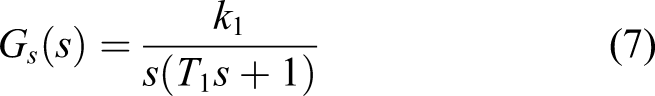
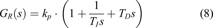
First, let us describe the property of the PID controller whose transfer function is:

G_{R} (s) = k_{p} · (1 + \frac{1}{T_{I} s} + T_{D} s)

(8)

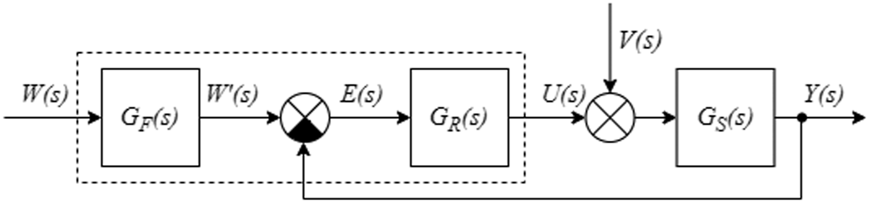
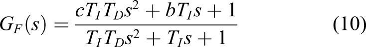
where k_P is the controller gain, and it is equal to the proportional (position) feedback, T_I is the integral constant of the controller, and the k_P/T_I is equal to the integration of the control error whose function is to obtain Y(s) = W(s) in the steady state. The last term is the derivative term containing the controller’s derivative constant T_D, where k_P · T_D is equal to the derivation (velocity) feedback.

The 2DOF controller has a similar structure. The only difference is the filter with the two constants b and c. Thanks to these parameters, we can control the influence of the setpoint variable compared to the output variable. The 2DOF controller can be described with the equation:

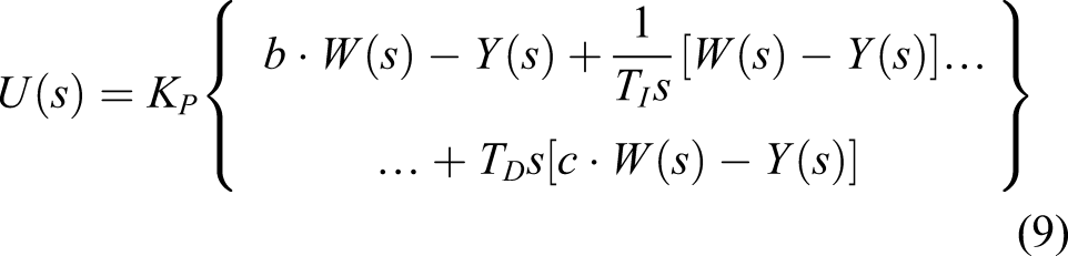
U (s) = K_{P} {\begin{matrix} b · W (s) - Y (s) + \frac{1}{T_{I} s} [W (s) - Y (s)] \dots \\ \dots + T_{D} s [c · W (s) - Y (s)] \end{matrix}}

(9)

If the b = 1 and c = 1, then the 2DOF controller is equivalent to the common PID controller. If the b = 0 and c = 0 then the filter is fully active. We can divide this controller into two blocks-the common PID controller and a separate filter. A final diagram can be seen in Figure 5. Then the transfer function of the filter is:

G_{F} (s) = \frac{c T_{I} T_{D} s^{2} + b T_{I} s + 1}{T_{I} T_{D} s^{2} + T_{I} s + 1}

(10)

Figure 5.

Closed loop control system with input filter.³

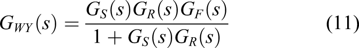
The transfer function of the setpoint to the output is equal to:

G_{W Y} (s) = \frac{G_{S} (s) G_{R} (s) G_{F} (s)}{1 + G_{S} (s) G_{R} (s)}

(11)

G_{W Y} (s) = \frac{k_{1} k_{p} (c T_{D} T_{I} s^{2} + b T_{I} s + 1)}{T_{1} T_{I} s^{3} + (T_{D} T_{I} k_{1} k_{p} + T_{I}) s^{2} + T_{1} k_{1} k_{p} s + k_{1} k_{p}}

(12)

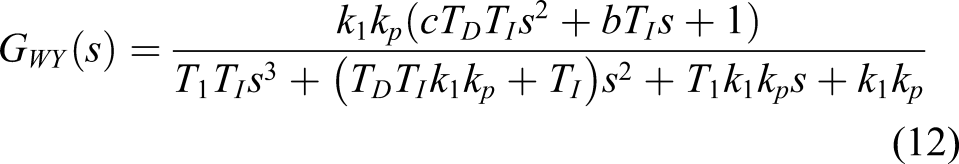
From this equation, we can see that using the conventional PID controller, we obtain two complex conjugated zeros. Their effect can be canceled using the 2DOF controller when $b = 0$ and $c = 0$ . If we set $b$ and $c$ to different non-zero or non-one, the zero can be altered.

If we use the substitution:

G_{P} (s) = \frac{k_{1} k_{p}}{T_{1} T_{I} s^{3} + (T_{D} T_{I} k_{1} k_{p} + T_{I}) s^{2} + T_{1} k_{1} k_{p} s + k_{1} k_{p}}

(13)

which is the transfer function of the proportional system, we obtain the transfer function from the setpoint to the output:

G_{W Y} (s) = G_{P} (s) + G_{P} (s) b T_{I} s + G_{P} (s) c T_{D} T_{I} s^{2}

(14)

The first term does not depend on any of the $b$ or $c$ parameters, the second term is the first derivation of the first term, and the influence can be controlled by the parameter $b$ , and the third term is the second derivation of the first term and can be controlled by the parameter $c$ . If $b$ or $c$ is negative, it can lead to the undershoot. $b$ parameter can be used to make the system response to the step setpoint change more aggressive. Parameter $c$ will have only a minimal influence on the dynamics of the system response to the step setpoint change. Visible differences will be noticeable right after the step setpoint change.

The transfer function of the disturbance to the output is equal to:

G_{v y} (s) = \frac{G_{S} (s)}{1 + G_{S} (s) G_{R} (s)}

(15)

G_{v y} (s) = \frac{T_{I} k_{1} s}{T_{1} T_{I} s^{3} + (T_{D} T_{I} k_{1} k_{p} + T_{I}) s^{2} + T_{1} k_{1} k_{p} s + k_{1} k_{p}}

(16)

As you can see, in the steady state $G_{v y} (s) = 0$ . Also, this transfer function is not affected by the 2DOF parameters $b$ and $c$ . The 2DOF PID controller used for the experimental verification in this paper is done by single chip computer implementation.³¹

Experimental identification of the integral plant

By direct identification with the step input signal, data describing the properties of the controlled system were obtained.

The measurement was performed by applying an input signal of 50% of the maximum range to the system input, and the step response of the system to this signal was recorded (see Figure 6). In the figure, the value of the output variable is normalized to the maximal angle of the rotation range. The same normalization is also used in the following paragraphs.

Figure 6.

DC motor output shaft angle of the rotation step response.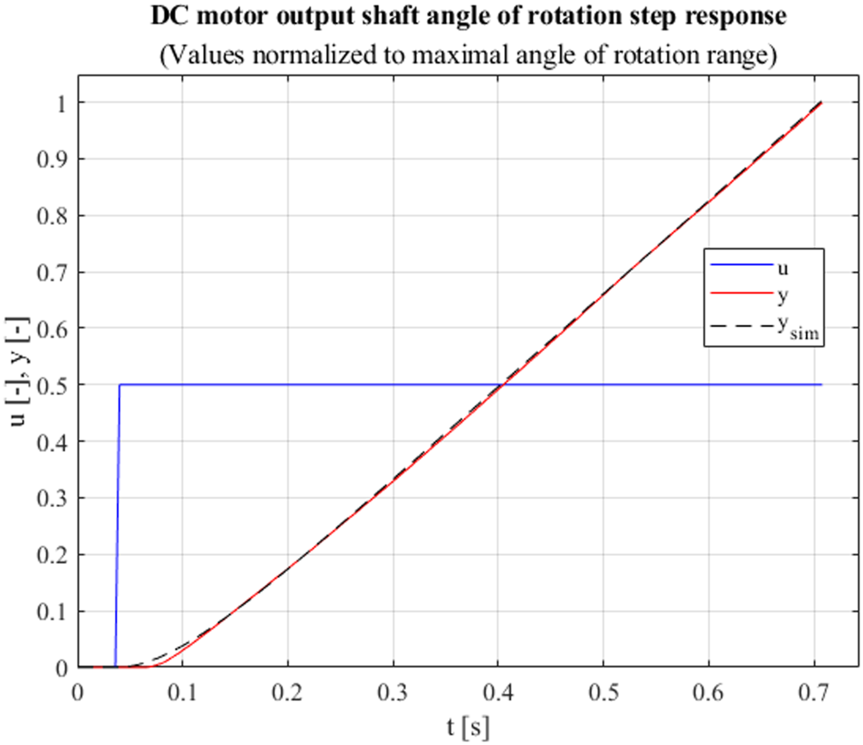

By processing the input data and normalizing the signals, the system’s transfer function was obtained in the form of an integration system with first-order inertia.

G_{S} (s) = \frac{1}{0.3039 s (0.0603 s + 1)} = \frac{3.2906}{s (0.0603 s + 1)}

(17)

Closed loop control

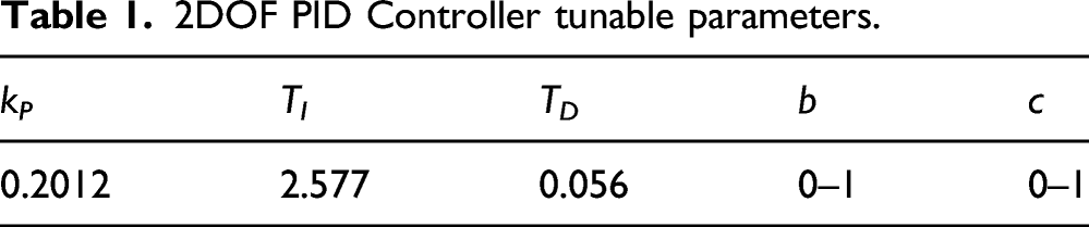
A control system was designed for the plant (system) described by (17) based on the previous theory. The PID controller parameters were tuned using the numeric optimization method, and they are listed in Table 1.

Table 1.

2DOF PID Controller tunable parameters.

k _P	T _I	T _D	b	c
0.2012	2.577	0.056	0–1	0–1

The experimental measurement was performed as a response to a step change of setpoint from the beginning of the measurement. At time t = 15 s, there was a step change of disturbance in front of the plant. The exact process was numerically simulated in the MATLAB /Simulink environment, where the identified system was controlled by a 2DOF controller with action variable limitation (see Figure 7). The parameters (weights) of the input filter were selected from the whole range 0–1 and measured and simulated with the step of 0.2. The disturbance is simulated by the software drop of action variable voltage on the input of the plant. The results of the measurements and simulations are plotted in Figure 8.^6,7

Figure 7.

MATLAB/Simulink numerical simulation schematic.

Figure 8.

Closed loop control (red – simulated, gray - measured).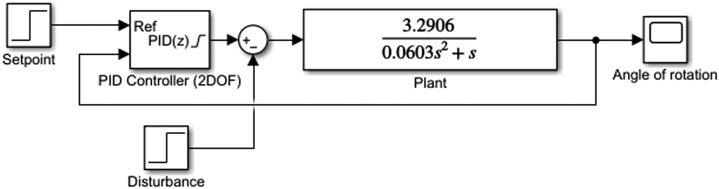

According to the results, the influence of the b parameter is significantly greater than the c parameter when tracking the setpoint in the form of the step. Proved also by the simulation, the b parameter suppresses the effect of proportional term and eliminates the overshoot of the control process while the response to a disturbance step remains unchanged.

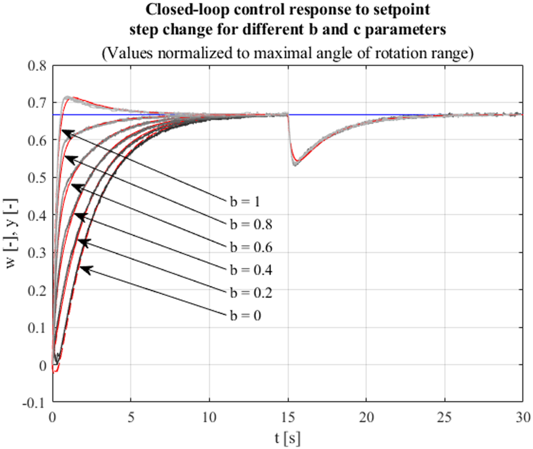
The effect of the individual terms according to (13) and (14) are shown in Figure 9. We split the three terms into separate courses that give the overall control system response using the same basic PID tunable parameters and b = 0.4 and c = 0.8.

Figure 9.

Comparison of the influence of the 2DOF terms (b = 0.4, c = 0.8).

Quality of feedback control

Multiple methods can be used to evaluate the quality of the feedback control. As it was described earlier, one of the expectations of the closed-loop control is that the transfer function of the setpoint to the output is equal to one. That also means that the error should be zero. For physical systems, we want the system error to minimize as fast as possible.

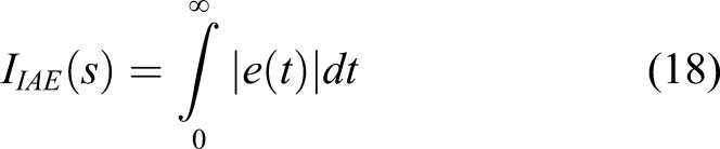
As an example, we can choose one of these criteria for evaluating the setpoint step change response course:

• Integral of Absolute Error (IAE)

I_{I A E} (s) = \int_{0}^{\infty} | e (t) | d t

(18)

• Integral of Squared Error (ISE)

I_{I S E} (s) = \int_{0}^{\infty} e^{2} (t) d t

(19)

• Integral of Time multiplied by Absolute Error (ITAE)

I_{I T A E} (s) = \int_{0}^{\infty} t | e (t) | d t

(20)

where a lower number means a faster control process. All these methods can be used for both non-oscillating and oscillating processes. The disadvantage of IAE and ITAE is that it cannot be calculated as a derivative of a zero-crossing for absolute value is not defined. Therefore, these methods can be calculated only numerically. The ISE is defined, but the oscillating processes have a lower error than non-oscillating processes. These methods are usually used for the quantitative methods of calculating the control variables as published in ^{9, 24}. We calculated the ITAE in this article. Numerical simulation is then compared to the measurements.

The calculated results for different parameters b and c can be seen in tables: measurements in Table 2 (ITAE) and numerical simulations in Table 3 (ITAE). Both the tables are plotted in the surface graph in Figure 10 and Figure 11 (simulated).

Table 2.

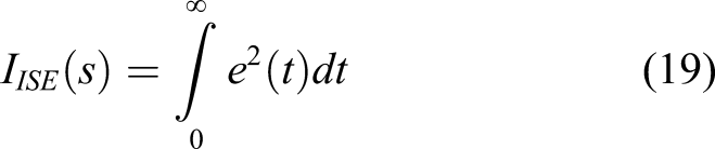
Quality of feedback control according to ITAE criteria.

b /c	0	0.2	0.4	0.6	0.8	1
0	11.46	11.54	11.58	11.36	11.41	11.35
0.2	10.37	10.36	10.52	10.26	10.48	10.45
0.4	9.35	9.37	9.35	9.45	9.47	9.31
0.6	8.36	8.41	8.39	8.19	8.40	8.45
0.8	7.33	7.36	7.28	7.33	7.44	7.31
1	7.09	7.07	7.12	7.16	7.08	7.40

Table 3.

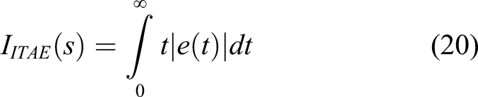
Quality of feedback control according to ITAE criteria (simulated).

b /c	0	0.2	0.4	0.6	0.8	1
0	11.09	11.10	11.10	11.10	11.10	11.10
0.2	10.11	10.12	10.12	10.12	10.12	10.12
0.4	9.13	9.14	9.14	9.14	9.14	9.14
0.6	8.15	8.16	8.16	8.16	8.16	8.16
0.8	7.17	7.18	7.18	7.18	7.18	7.18
1	7.09	7.08	7.08	7.08	7.08	7.08

Figure 10.

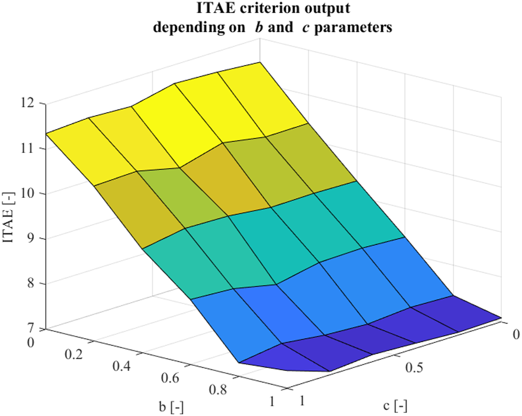
Results of the ITAE criterion for different b and c parameters.

Figure 11.

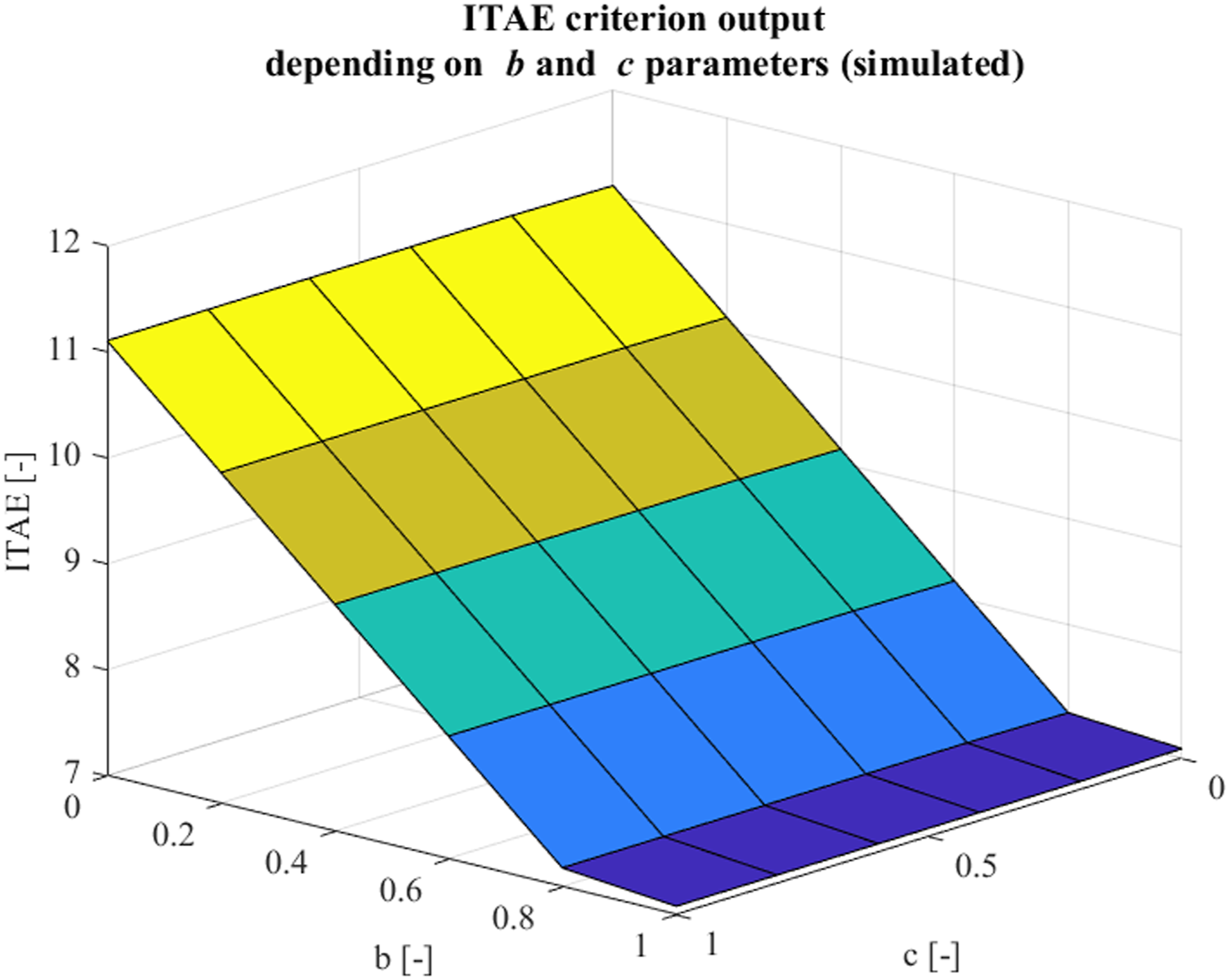
Results of the ITAE criterion for different b and c parameters (simulated).

As we can see from the results, the differences between the simulation and measurements containing small nonlinearities are neglectable. The parameter $c$ has only a tiny influence on the quality, while lowering the $b$ parameter slows down the response. The response to the disturbance is not affected by the 2DOF controller parameters as stated above.

Using an input 2DOF filter, suppression of the overshoot of the control process course is achieved, while without it, the control process course shows an overshoot of approximately 7% at a given setting.

Conclusion

The paper shows that using the 2DOF controller, we obtain more flexibility in designing the final desired system response. The theory was implemented into the Arduino-based control system experimentally identified and controlled by the 2DOF PID controller.

The transfer function for setpoint tracking and the reaction of the output to the disturbance was calculated for the integral system with the first-order inertia. The closed-loop control using the typical PID controller contains two zeros, which for the integral system makes the response more aggressive from the beginning after the setpoint step change. That leads to fast elimination of the disturbance change but causes an overshoot. This behavior can be suppressed using the 2DOF PID controller, where these zeros can be canceled by setting the $b$ and $c$ parameters to lower values. Using the $b$ or $c$ parameters, we can also design the dynamics of setpoint tracking without affecting the behavior of the closed-loop control system to the disturbances.

The measurement and simulation proved that the overall influence of the b parameter is considerably more dominant when tracking the setpoint value. According to the criteria used to evaluate the quality of the control process, you can conclude that the settling time is not significantly extended (if we consider a sufficiently narrow tolerance band). However, the setpoint step function response overshoot is suppressed, which can be very important for some dynamic systems. Depending on the settings of the 2DOF filter parameters, we can then achieve an overshoot-free course while maintaining the same settling time. In the case of the particular system used, this setting is around the value 0.8–0.9 for parameter b.

Footnotes

Declaration of conflicting interests

The author(s) declared no potential conflicts of interest with respect to the research, authorship, and/or publication of this article.

Funding

The author(s) disclosed receipt of the following financial support for the research, authorship, and/or publication of this article: This work was supported by the European Regional Development Fund in the Research Centre of Advanced Mechatronic Systems project, CZ.02.1.01/0.0/0.0/16_019/0000867 within the Operational Programme Research, Development and Education and the project SP2022/60 Applied Research in the Area of Machines and Process Control supported by the Ministry of Education, Youth and Sports.

ORCID iDs

Radek Guras

Miroslav Mahdal

References

Guras

Mahdal

Nonlinear integral system control

[online]. In: 2020 21th International Carpathian Control Conference (ICCC), 2020, Košice, Slovak Republic, 2020-10-27, pp. 1–4. [cit. 2021-7-15]. DOI: 10.1109/ICCC49264.2020.9257237

Kaya

. A PI-PD controller design for control of unstable and integrating processes. ISA Trans 2003; 42(1): 111–121, [cit. 2021-9-9]. DOI: 10.1016/S0019-0578(07)60118-9.

Simhachalam

Dey

Mudi

. An auto-tuning PD controller for DC servo position control system. [online]. 2012 2nd Int Conf Power Control Embedded Syst 2012; 2012: 1–6, [cit. 2021-9-9]. DOI: 10.1109/ICPCES.2012.6508121.

PEKER, Fuat a Ibrahim KAYA . Identification and real time control of an inverted pendulum using PI-PD controller [online]. In: 2017 21st International Conference on System Theory, Control and Computing (ICSTCC), Sinaia, Romania, 19-21 October 2017. IEEE, 2017, pp. 771–776. [cit. 2021-9-9]. DOI: 10.1109/ICSTCC.2017.8107130.

O'dwyer

. Handbook of PI and PID controller tuning rules . 3rd edition. Hackensack, NJ: Distributed by World Scientific Pub., 2009.

Chidambaram

Padma Sree

. A simple method of tuning PID controllers for integrator/dead-time processes. [online]. Comput Chem Eng 2003; 27(2): 211–215, [cit. 2021-9-9]. DOI: 10.1016/S0098-1354(02)00178-3.

Astrom

Hagglund

. Advanced PID control. Research Triangle Park, NC: ISA-The Instrumentation, Systems, and Automation Society, 2006.

Sladka

Guras

Viteckova

Position control with 2DOF PI controller

[online]. In: 2020 21th International Carpathian Control Conference (ICCC), Shah Alam, Malaysia, 27 October, 2020, 2020, pp. 1–4. [cit. 2021-7-15]. DOI: 10.1109/ICCC49264.2020.9257260

Viteckova

Vitecek

. 2DOF PID controller tuning for integrating plants. [online]. In: 2016 17th International Carpathian Control Conference (ICCC), High Tatras, Slovakia, 29 May-1 June 2016, IEEE, 2016, pp. 793–797. [cit. 2021-7-15]. DOI: 10.1109/CarpathianCC.2016.7501204.

10.

Lunze

. PID-Regelkreise mit zwei Freiheitsgraden. [online]. At - Automatisierungstechnik 2021; 69(7): 565–573, [cit. 2021-8-26]. DOI: 10.1515/auto-2021-0006.

11.

Zhong

Q-C

Normey-Rico

. Control of integral processes with dead-time. Part 1: Disturbance observer-based 2DOF control scheme. [online]. IEE Proc - Control Theor Appl 2002; 149(4): 285–290, [cit. 2021-8-26]. DOI: 10.1049/ip-cta:20020438.

12.

Vilanova

Serra

Realisation of two-degrees-of-freedom compensators. [online]. IEE Proc - Control Theor Appl 1997; 144(6): 589–595, [cit. 2021-8-26]. DOI: 10.1049/ip-cta:19971617.

13.

Alfaro

Vilanova

. Two-degree-of-freedom PID controllers structures. Model-Ref Robust Tuni PID Controllers. [online]. Cham: Springer International Publishing, 2016. 2016-04-17, 7-19 [cit. 2021-8-26]. Advances in Industrial Control. DOI: 10.1007/978-3-319-28213-8_2.

14.

Taguchi

Araki

. Two-degree-of-freedom PID controllers - their functions and optimal tuning. [online]. IFAC Proc Volumes 2000; 33(4): 91–96, [cit. 2021-7-15]. DOI: 10.1016/S1474-6670(17)38226-5.

15.

Hirahara

Tanaka

Yamamoto

, et al. Systematic design of two-degree-of-freedom PID controller for positioning and tracking drives of linear servo motors. [online]. IEEJ J Industry Appl 2017; 6(6): 443–448, [cit. 2021-8-26]. DOI: 10.1541/ieejjia.6.443.

16.

Wang

Yan

, et al. An approach for setting parameters for two-degree-of-freedom PID controllers. [online]. Algorithms 2018; 11(4): 48. DOI: 10.3390/a11040048. [cit. 2021-8-26]

17.

Hassaan

Tuning of a Feedforward 2DOF PID Controller to Control Second Order-Like Processes

[online]. 2018, [cit. 2018-12-17]. Availabe from: http://oaji.net/articles/2017/1992-1537361127.pdf

18.

Deshmukh

GL.

Kadu

. Design of two degree of freedom PID controller for temperature control system. In: 2016 International Conference on Automatic Control and Dynamic Optimization Techniques ICACDOT, Pune, India, 9-10 September 2016, 2017, pp. 586–589. art. no. 7877653.

19.

Shi

, et al. Active disturbance rejection control design for high-order integral systems. [online]. ISA Trans 2021, [cit. 2021-9-9]. DOI: 10.1016/j.isatra.2021.06.038.

20.

Han

. From PID to active disturbance rejection control. [online]. IEEE Trans Ind Electronics 2009; 56(3): 900–906, [cit. 2021-9-9]. DOI: 10.1109/TIE.2008.2011621.

21.

Zhao

Z-L

Guo

B-Z

. On convergence of nonlinear active disturbance rejection control for SISO nonlinear systems. [online]. J of Dynamical Control Syst 2016; 22(2): 385–412, [cit. 2021-9-9]. DOI: 10.1007/s10883-015-9304-5.

22.

Sariyildiz

Oboe

Ohnishi

. Disturbance observer-based robust control and its applications: 35th anniversary overview. [online]. IEEE Trans Ind Electronics 2020; 67(3): 2042–2053, [cit. 2021-9-9]. DOI: 10.1109/TIE.2019.2903752.

23.

Ding

Chen

W-H

Mei

, et al. Disturbance observer design for nonlinear systems represented by input-output models. [online]. IEEE Trans on Ind Electronics 2020; 67(2): 1222–1232, [cit. 2021-9-9]. DOI: 10.1109/TIE.2019.2898585.

24.

Sladka

Viteckova

. 2DOF PI controller tuning for integrating plants with the setting of setpoint weight. [online]. In: 2019 20th International Carpathian Control Conference (ICCC), Krakow-Wieliczka, Poland, 26-29 May 2019, 2019: 1–4, [cit. 2021-11-23]. DOI: 10.1109/CarpathianCC.2019.8765989.

25.

Huba

. Comparing 2DOF PI and predictive disturbance observer based filtered PI control. [online]. J of Process Control 2013; 23(10): 1379–1400. [cit. 2021-9-9]. DOI: 10.1016/j.jprocont.2013.09.007.

26.

Azid

Shankaran

Mehta

. Fractional PI controller for integrating plants. [online]. In: 2020 16th International Conference on Control, Automation, Robotics and Vision (ICARCV), Shenzhen, China, 13 December, 2020, 2020, pp. 904-909 [cit. 2021-11-23]. DOI: 10.1109/ICARCV50220.2020.9305506

27.

Gozde

. Robust 2DOF state-feedback PI-controller based on meta-heuristic optimization for automatic voltage regulation system. [online]. ISA Trans 2020; 98: 26–36, [cit. 2021-11-23]. DOI: 10.1016/j.isatra.2019.08.056.

28.

Zhang

. An improved 2-degree-of-freedom internal model proportional-integral-derivative controller design for stable time-delay processes. [online]. Meas Control 2020; 53(5–6): 841–849, [cit. 2021-11-23]. DOI: 10.1177/0020294020912522.

29.

Padiachy

Mehta

Azid

, et al. Two degree of freedom fractional PI scheme for automatic voltage regulation. [online]. Eng Sci and Technol Int J 2022; 30: 101046, [cit. 2021-11-23]. DOI: 10.1016/j.jestch.2021.08.003.

30.

Czebe

Skuta

. Usage of single-chip computers for control MIMO systems. In: 2017 18th International Carpathian Control Conference (ICCC), Sinaia, Romania, 28-31 May 2017. [online]. IEEE, 2017, pp. 369–374. [cit. 2021-7-15]. DOI: 10.1109/CarpathianCC.2017.7970428.

31.

Sladka

Czebe

Wagnerova

. The 2DOF controller implementation in control system with single-chip computer. In: 2018 19th International Carpathian Control Conference (ICCC), Szilvasvarad, Hungary, 28-31 May 2018, [online], 2018: pp. 228–234. IEEE. [cit. 2021-11-23]. DOI: 10.1109/CarpathianCC.2018.8399633.

The PID and 2DOF control of the integral system - influence of the 2DOF parameters and practical implementation

Abstract

Keywords

Introduction

Description of the system

Theory of the 2DOF PID controller

Experimental identification of the integral plant

Closed loop control

Quality of feedback control

Conclusion

Footnotes

Declaration of conflicting interests

Funding

ORCID iDs

References