
Abstract
This paper explores the concept of interactive perception, in which sensing guides manipulation, in the context of extracting and classifying unknown objects within a cluttered environment. In the proposed approach, a pile of objects lies on a flat background, and the goal of the robot is to isolate, interact with, and classify each object so that its properties can be obtained. The algorithm considers each object to be classified using color, shape, and flexibility. The approach works with a variety of objects relevant to service robot applications, including both rigid objects such as bottles, cans, and pliers as well as non-rigid objects such as soft toy animals, socks, and shoes. Experiments on a number of different piles of objects demonstrate the ability of efficiently isolating and classifying each item through interaction.
1. Introduction
Humans routinely shuffle through papers on a desk or sift through objects in a drawer to more quickly and efficiently identify items of interest. In such cases, it is our interaction with the environment that increases our understanding of the surroundings, in order to more effectively guide our actions to achieve the desired goal. In a similar manner, animals such as racoons and cats are known to use their front paws to poke and swat at objects to better understand them, whether it involves playing with a toy or trying to catch a rodent [28]. During such interaction, one mode of information acquisition is obviously contact sensing, i.e., haptics, but a potentially richer source of information is also available via vision.
Brock and colleagues [11], [12] have recently introduced the term “interactive perception” to describe a system in which a robot learns about the environment by interacting with it. Video from a stationary camera is used to locate and track objects as they move around a table as a result of poking and prodding by a robot arm. Interactive perception is a new approach towards autonomous manipulation. Rather than separating action from perception and solving each independently, this new methodology argues they should both be interleaved so that they can benefit from one another in a more tightly coupled way.
Inspired by the above work, this paper introduces a new approach to interactive perception (which we also call “manipulation-guided sensing”), in which successive manipulations of objects in an environment are used to increase vision-based understanding of that environment, and vice versa. See Figure 1. The motivation for this work includes not only the extraction of harmless objects such as a sock in a drawer but also the discovery of delicate and possibly dangerous objects that are initially hidden from the field of view. For example, in searching for an explosive device a robot must be careful to gently remove the obstructing objects while disturbing the rest of the pile as little as possible. This paper extends our previous work [30] by incorporating an object extraction algorithm, similar to [31], and applying the system to a recycling scenario involving metal cans and plastic bottles. The paper demonstrates the usefulness of interactive perception in solving the problem of retrieving an object within a cluttered pile, as well as classifying it for future interactions. We show that deliberate actions can change the state of the world in a way that simplifies perception and consequently future interactions.

The proposed setting for manipulation-guided sensing. Left: A robotic arm interacts with a pile of unknown objects (soft toy animals) to segment the individual items one at a time. An overhead stereo pair of cameras (Logitech QuickCam Pro webcams) is used. Right: The system then learns about each object's characteristics by automatically isolating it from the pile and interacting with it. A third overhead camera is used for sensing the isolated object.
2. Previous work
Early work in interactive perception was performed by Christensen and Nørgaard [4], who developed an autonomous system to autonomously learn the physical properties of an unknown object by colliding with a mobile robot and tracking the resulting trajectories using an overhead camera. A similar approach was performed by Fitzpatrick [7], who showed that visual segmentation of an object is greatly improved when a robotic manipulator is allowed to poke an object and observe the resulting motion. Another approach to active segmentation focuses on performing foreground/background segmentation in an image given a fixation point [17], an idea that falls within the general paradigm of active vision [1].
More recent work in interactive perception has been addressed by Brock and colleagues. Katz and Brock [11] describe a system in which a manipulator learns about the environment by interacting with it. Video available from an overhead camera is analyzed by tracking feature points on an object in order to determine the number, location, and type (revolute or prismatic) of joints on an articulated object lying on a table. In followup work, Kenney et al. [12] developed an interactive system in which a robotic arm interacts with objects on a table, and an overhead camera captures the scene. The video is used to subtract the current image from the previous image to locate and track objects as they move around the table as a result of the interaction. Our work differs in its purpose and scope. Rather than recovering geometric properties of a single unobstructed rigid articulated structure, our concern is with sifting through a cluttered pile of objects, many of which are occluding one another, and properly classifying each object. In this way, our work bears some similarity to classification based on affordance cues [25]. Unlike [11], [12], our objects can be either rigid or non-rigid, and our results provide a skeleton of the object along with some geometric properties to more fully aid classification.
Other related work is that of Saxena et al. [22], in which information about a scene is gathered to generate a 3D model of each object present. The 3D model is then compared against a database of previously created models with grasping locations already determined. While this approach does involve learning models of objects, it relies on a previously recorded database rather than interleaving manipulation with perception. Our method is different in that the objects in the pile being examined in this work are unknown a priori, so we do not have access to a database of the objects being examined.
Other researchers have pursued this idea of interacting with an object by pushing, tapping, or grabbing to discover attributes of the object. In [13] [18], for example, a robot was used to interact with a ball. When an operator informed the robot that the ball was a certain color and that it rolls when “pushed,” the robot learned about the particular color and the meaning of the word “rolling” by matching the operator input with the observations of the object after interaction. In [18], the robot captured the object's reaction to one of three interactions: “grasp”, “tap”, or “touch”. The robot was then used to imitate what it had learned from interacting with the object. In [24], the problem of learning about visual properties and spatial relations was addressed, using vision, communication, and manipulation subsystems. Our work coincides with the same goal as these approaches but without using communication or verbal input from an operator.
Our approach is aimed at handling both rigid and non-rigid objects. This goal fits well with the needs of service robots that must operate in unstructured environments. In particular, previous work involving service robot applications has been geared towards grasping [9] and folding clothes [21] [19].
Clothing is highly non-rigid, and manipulating and interacting with non-rigid objects is still a largely unsolved problem for robotics, although some notable progress has been made in recent years [19], [16], [15], [9], [34], [21], [5], [20], [14], [32], [31], [33], [29].
3. Extracting and isolating objects
Our approach is divided into two phases, as shown in Figure 2. The goal of Phase 1 is to extract a single item from a pile of unknown objects, while Phase 2 comprises of classifying the unknown object. We now describe Phase 1 in detail. Graph-based segmentation [6] starts the process to divide the area into regions based on color. Next, stereo matching is used to determine the initial region in which to concentrate. After the selected region is chosen from the graph-based segmentation and stereo matching, a grasp point is selected to determine where and how to extract the object. Lastly, the manipulator sets the object aside to be classified to aid identification and manipulation of the object in future interactions.

Overview of our entire system for vision-guided extraction and classification of a pile of unknown objects.
To determine if there are no more objects in the scene, the currently selected region is tested whether it is smaller than a predetermined threshold of bmin, which was computed as the average size of the graph-segmentation regions corresponding to the top object. If the region is less than bmin, then the algorithm decides that there are no more objects in the image since the objects in our scenarios are on average larger than a size of bmin.
A. Graph-based segmentation
Graph-based segmentation [6] is an algorithm used to take an image and segment it into different regions based on feature vectors associated with the pixels (e.g., color). This algorithm forms the first step in the extraction process. Figure 3 shows the results of graph-based segmentation on an example image taken in our lab. The graph-based segmentation gives a layout of the original image broken up into various regions. Those regions are then examined to calculate the area of each region, whether the region is touching the border of the image, and the mean color value in the region.

LEFT: An image taken in our lab. RIGHT: The results of applying the graph-based segmentation algorithm. Despite the over-segmentation, the results provide a sufficient representation for grasping the object.
Our initial goal is to determine which object is on top of the pile, so that a single object can be extracted from the scene while minimizing the chance of disturbing the surrounding objects. There are many monocular image cues that can provide a hint as to which object is on top, such as the size of the object, its concavity, T-junctions, and so forth. The graph-based segmentation facilitates the separation of background and foreground regions, thereby removing the former from consideration. The background is considered to be all the colors associated with pixels located on the border of the image. To decide among the foreground, we rely upon stereo matching using a pair of cameras. The idea behind looking for the object on top of a pile is so that the other regions (or objects) in the pile would not be disturbed when extracting the selected region.
B. Stereo matching
Stereo matching is the process in visual perception leading to the sensation of depth from two slightly different projections of an environment [23]. With rectified cameras, the difference in image coordinates between two corresponding points in the two images arise from the cameras' different positions along the baseline. This image difference is called horizontal disparity, and it is inversely proportional to the distance from the camera to the point. We implemented a window based sum-of-absolute differences (SAD) stereo algorithm [23] for its computational efficiency, utilizing MMX/SSE2 SIMD operations to increase the speed of computation. The disparity image that results from stereo matching is used to estimate the relative distance to each segmented area found in the previous section.
The disparity image contains noise from misalignment of the cameras, reflections in the scene (non-Lambertian surfaces), and occlusion. To reduce the effects of this noise, we employ a left-right consistency check [8] to retain only those disparities that are consistent in both directions. We also use the graph-based segmentation image to separate the background from the foreground. Among the foreground disparities, connected constant-disparity regions whose area exceeds a threshold, amin, are retained while smaller regions are discarded. (We set amin = 0.04% of the image.) Figure 4 shows the results of the stereo matching before and after reducing the effects of noise. Photometric inconsistency between the cameras is handled by adjusting the gain of one image to match the other.
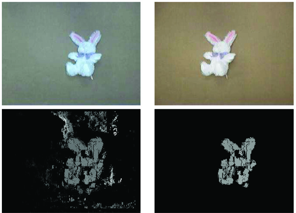
TOP: A stereo pair of images taken in our lab, showing the large amount of photometric inconsistency. BOTTOM: The disparity image obtained by SAD matching (left), and the result after masking with the foreground and removing small regions (right).
C. Determining grasp point
Determining the grasp point is a critical step for picking up the selected object. If the object itself or surrounding items are fragile or sensitive, then it is important to minimize the amount of disturbance. Because some of our objects are non-rigid and irregularly shaped, we cannot use the approach of [22] because they only involve rigid objects and train their system from a database of known objects. Instead, we calculate the 2D grasp point as the geometric center of the object, defined as the location whose distance to the region boundary is maximum. This point, which can be computed efficiently using chamfering [3], is much more reliable than the centroid of the region, particularly when the region is concave. The nature of the objects and grasp scenarios considered in this paper motivates contact at their geometric center.
Figure 5 shows the grasp point found by the maximum chamfer distance for a selected object. Once the grasp point has been found, the robot arm is moved over the pile of objects, the end effector is positioned above the grasp point, the arm is positioned two inches away from the expected height given by the stereo cameras, and the arm lowers the end effector orthogonally to the image plane to grab the object and remove it from the scene. The arm is positioned closely to the expected height because when the arm is lowered in the orthogonal direction, the trajectory generator used in the robotic computer adds a small curvature to move from one point to another.

LEFT: The binary region associated with an object. The grasp point (red dot in the center) is the location that maximizes the chamfer distance. RIGHT: The chamfer distance of each interior point to the object boundary.
Once the arm has retreated from the camera's field of view, the images before and after the extraction procedure are compared to determine whether, in fact, the object was removed. This decision is made by comparing the number of pixels whose absolute difference in intensity exceeds a threshold and the size of the object. As long as the object has not been successfully removed, the arm is successively lowered a small amount to try again, until either the object is taken or the end effector has reached a maximum distance (to avoid collision with the table on which the object is sitting). These repeated attempts overcome the lack of resolution in our stereo imaging configuration. The extraction process continues until all of the objects in the image have been removed (i.e., when all of the segmented image regions that do not touch the image boundary are smaller than the minimum threshold, bmin).
4. Classifying and labeling objects
Phase 2 is the classification and labeling process, which begins with color histogram labeling [26], which enables the item to be identified based on its distribution of red, green, and blue color values. The next step is skeletonization, which provides a 2D model of the unknown object to be used in determining locations of revolute joints and interaction points. Once the skeleton is constructed, the robotic arm interacts with the object to further study it while monitoring the object interaction by observing the object's reaction to the robotic arm's involvement. Finally, labeling revolute joints using motion uses the monitored interactions to determine joints on the object that are movable and others that are rigid. After the final step, a revised skeleton is created with the revolute joints labeled. This revised skeleton provides a more accurate model of the unknown object and also aids in calculating a grasp point and orientation.
A. Color histogram labeling
When an object has been extracted from the pile, it is set aside in order to study it further. This procedure involves constructing a model of the object and comparing that model with the models (if any) of previous objects that have been encountered. To compare objects we use a color histogram, both for its simplicity and for its robustness to geometric deformations. A color histogram is a representation of the distribution of colors in an image, derived by counting the number of pixels with a given set of color values [26]. The color space is divided into discrete bins containing a range of colors each. We use eight bins for each color range of red, green, and blue, leading to 512 total bins.
Objects are matched by comparing their color histograms. For this step, we use histogram intersection [26], which is conveniently affected by subtle differences in small areas of color while at the same time being guided by the dominant colors. The histogram intersection is normalized by the number of pixels in the region, leading to a value between 0 and 1 that can be interpreted as the probability of a match. By comparing the color histogram of the currently isolated object with histograms of previously encountered objects, we are able to determine the identity of the object. If the probability is high enough, then the objects are considered to be the same; otherwise, the current object has not been seen before and its histogram is therefore added to the database. (We set the minimum probability for this decision to be 70%.) Figure 6 shows the isolated object to be classified, along with its binary mask.

LEFT: The isolated object to be classified. RIGHT: The binary mask of the object used in constructing its color histogram model.
B. Skeletonization
Skeletonization is the process of determining the internal structure of an object. Skeletonization can be described using the prairie-fire analogy: Setting the boundary of the object on fire, the skeleton is the loci where the fire fronts meet and quench each other [2]. The skeleton representation illustrates the locations of the extremities or limbs of the object. The locations where the extremities meet the torso or innermost line are considered intersection points, while locations where extremeties begin are considered end points. The intersection points are the initial guesses of the locations of the object's joints. End points are positions that are used to interact with the robotic arm. Figure 7 gives an example of a soft toy animal with its skeleton.

LEFT: The original object. MIDDLE: The isolated object to be classified. RIGHT: The skeleton of the object.
C. Monitoring object interaction
Monitoring object interaction involves tracking feature points within an image to understand the movements and overall makeup of the object. This process is facilitated by using the Kanade-Lucas-Tomasi (KLT) feature tracker [27]. The KLT algorithm selects feature points in an image and then maintains their location in the image as they move due to scene changes resulting from camera or object motion. Detecting features in the image is used when the selected region is found by separating the foreground from the background using graph-based segmentation.
After the KLT algorithm provides features within the whole image, only the features within the selected region are kept, and the other features are discarded. Figure 8 shows the KLT features for the whole image on the left and only the features within the selected region on the right. Before KLT feature detection is applied, the region is dilated to include the features along the edge of the object. Finally, the end points mentioned previously are used to instruct the arm where to interact with the object.
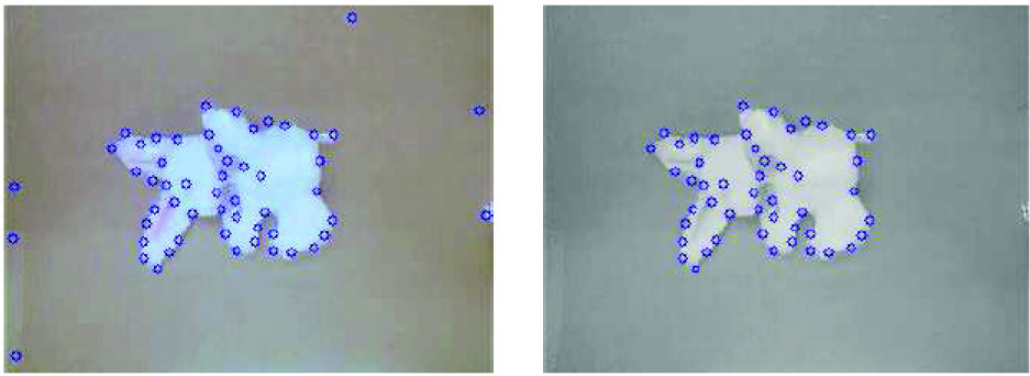
LEFT: KLT features selected in the whole image. RIGHT: Features that are located within the region selected by graph-based segmentation.
The arm interacts with the object by pushing at each end point orthogonal to the object. The end effector of the arm is placed two inches away from the object in the direction of the vertical or horizontal axis of the image plane, depending on the location of the end point. End points are compared with one another to determine if they are close to each other, determined by their Euclidean distance being below a threshold of 5. The remaining end points are grouped based on whether the point is closer to the top of the image or to the left of the image. If the former, then the end effector moves in the vertical direction of the image plane, otherwise it moves in the horizontal direction of the image plane.
As the arm interacts with the object, the algorithm groups various clusters of features based on distance and direction values. The process then checks to see if the current number of frames in the video feed from the camera is a multiple of flength. If the number is a multiple of flength, then the algorithm segments parts of the image using the clustering algorithm. If not, then it continues monitoring the item. In our experiments, we set flength to be 5 frames.
Figure 9 shows an example of clustering feature points. On the left side, the figure shows the feature points of the original object before clustering occurs. On the right side, the figure shows the feature points after flength frames of video and the separation of two different groups. The boundary line indicates the distances between the two groups that are greater than the prespecified threshold of 10.

Example of clustering feature points according to inter-distance values, in Euclidean space. (a) Before clustering and (b) after clustering with decision boundary.
In the work of [11], small groups with three or fewer features are discarded from the image. However, in our approach we have found that such groups hold some significant value in the case that some feature points attached to the object have been lost, resulting in a small group of features remaining. Therefore, in our algorithm all groups with at least two features are retained. As for groups of size one, the single feature point is then attached to the nearest group, using the Euclidean distance in the image.
D. Labeling revolute joints using motion
Labeling revolute joints using motion coincides with the monitoring process using KLT tracking. The features are clustered based on the Euclidean distances between them in the image plane. Features with similar motion vectors have relatively constant inter-feature distances and are therefore placed in the same group, while features with different motion vectors are separated into distinct groups.
After the selected region has been divided into one or more groups, an arbitrary feature point in each group is analyzed to decide if that group has moved more than the rest of the groups in the image. The assumption is that the interacted region is moving, while the other areas remain relatively stationary. The group whose computed motion is greater than the prespecified threshold is then determined to be movable and connected to a revolute joint.
If the feature group size is larger than one, then the surrounding ellipse of the feature group is used to calculate the end points along the major axis, illustrated in Figure 10, using principle component analysis (PCA) [10]. The end points of the major axis are considered the location of the revolute joint and the end of the rigid link. If the feature group size is only one point, then the intersection point closest to that feature is considered to be a revolute joint. Figure 11 gives an example of the mapping between feature points and intersection points within an image.

Example of grouping feature points to locate revolute points near the endpoints of the major axis.

Example of mapping feature points to the nearest intersection point.
Figure 12 illustrates the initial skeleton labeled with intersection points and end points and the revised skeleton with revolute joints labeled after several interactions with the robotic arm. The new skeleton is designed with movable joints labeled and all other joints deemed rigid. The end points associated with rigid joints are removed because any branches that do not have a revolute joint are considered noise in the skeleton. Only branches with movable joints are considered extremities of the object.

LEFT: The original skeleton. MIDDLE: Skeleton with intersection points and end points labeled. RIGHT: Revised skeleton after multiple interactions.
5. Experimental results
A. Platform
The proposed approach was applied in a number of different scenarios to test its ability to perform practical interactive perception. These scenarios were created to simulate real world experiences and interactions. A PUMA 500 robotic arm was used in these experiments, along with Logitech QuickCam Pro webcams. In each experiment, a pile of objects rested upon a flat, uniform background. The objects themselves, their type, and their number were unknown beyond being above a specific minimum size.
The results of the system are displayed below at different steps of the algorithm to show the robot's view, which object was selected for extraction, and the results of interacting with the object. With each step the algorithm finds a selected object to first extract. The robot arm is then sent to the grasp point to take the object out of the picture and isolate it. The system then labels the object based on its color. Next, the arm interacts with the object at calculated areas based on the skeleton of the object. Finally, a 2D model of the object is created after monitoring the feature points on the object.
B. Extraction and isolation experiment
Figures 13 and 14 show the individual steps resulting from an experiment involving four soft toy animals in a pile. The image was segmented, the algorithm found an object and determined a grasp point, then the robot grasped the object and set it aside to a predetermined location to the left of the pile (below the third camera). After a color histogram model of the object was constructed, a skeleton of the object was created to locate possible points of interaction and revolute joints. The robot then poked the object at calculated locations and monitored the movement of the object in response to the robot's interaction. After a final skeleton was determined, the object was removed from the field of view. The process was then repeated as the system found, extracted, and examined each object in turn, until there were no more objects remaining in the pile.
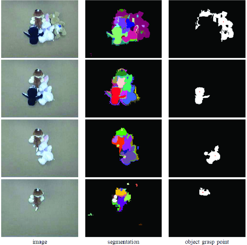
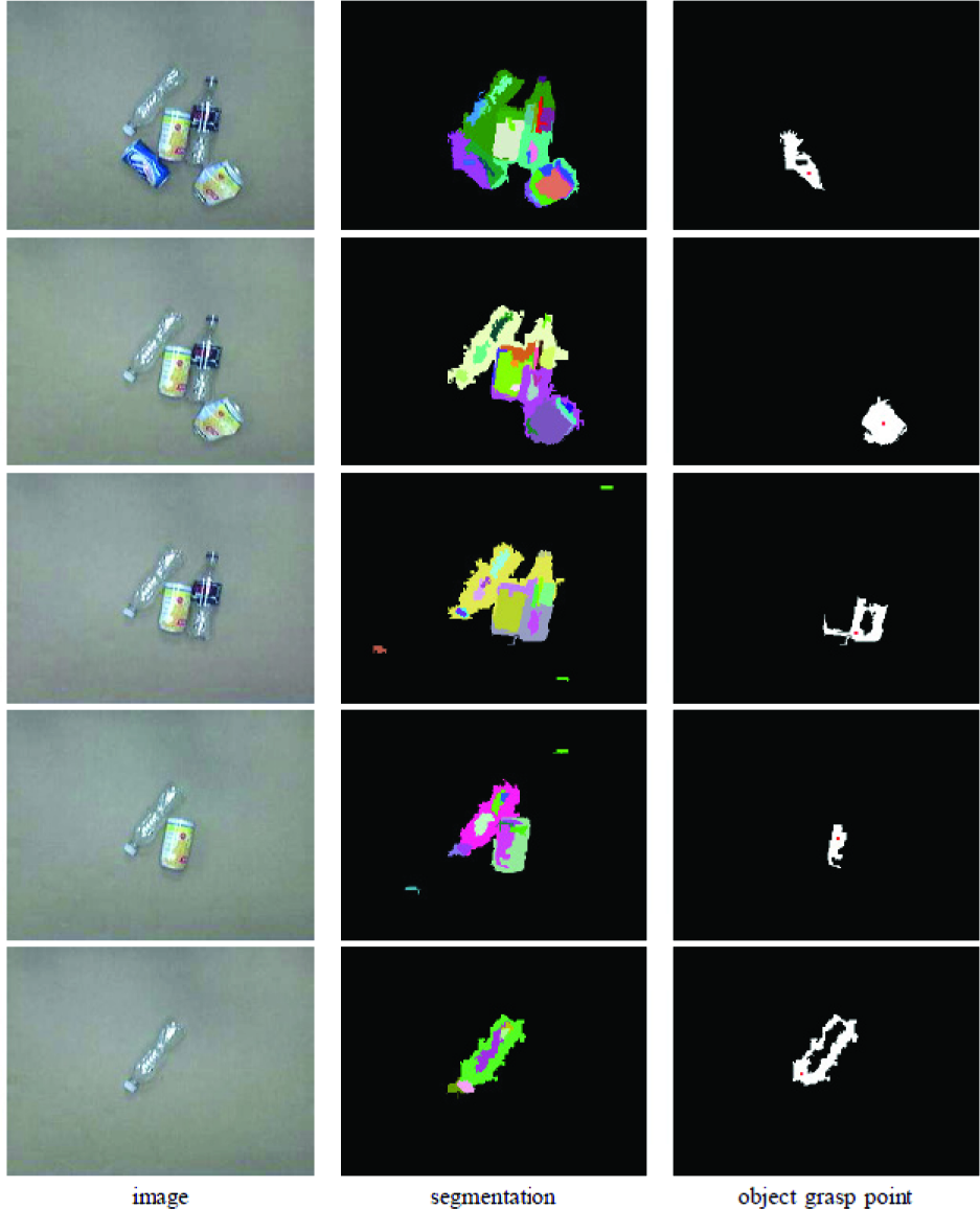
An experiment involving a pile of four unknown objects. From left to right: The image taken by the left camera, the result of graph-based segmentation, and the object found along with its grasp point(red dot). Time flows from top to bottom, showing the progress as each individual object is located and extracted.

From left to right: The image, taken by the third camera, after the object has been isolated, the binary mask of the isolated object, the skeleton with the intersection points and end points labeled, the feature points gathered from the isolated object, the image after mapping the feature points to the intersections points, and the final skeleton with revolute joints labeled. Time flows from top to bottom, showing the progress as each individual object is examined.
C. Classification of soft toy animals
We repeated the experiment with a larger set of eight unknown soft toy animals to demonstrate the classification process and the possible uses of labeling individual objects for further learning. Each time an object was extracted, the system captured an image of the isolated object, along with its binary mask and final skeleton. Figure 15 shows the eight images that were gathered automatically by the system as the objects were removed from the pile. The mask shows which pixels within the image were used for constructing the color histogram. The skeleton shows the 2D outline model of the object along with the revolute joints.

TOP: Images of the individual objects extracted automatically. MIDDLE: The binary masks used for building the color histograms of the objects. BOTTOM: The final skeletons with revolute joints labeled.
After the database of histograms was built, the objects were randomly rearranged in a new pile to test the classification performance of the system. As the objects were extracted again from the new pile, the color histogram of each object was compared against the database to determine the most likely match. If more than one color histogram was larger than Thmin, then the skeleton was used as a second form of classification to further identify the object (we set Thmin to 70%). Information calculated from the skeleton that could be used to further separate unlike objects are the number of extremities, or the number of revolute/non-revolute joints. During the experiments reported here, only the number of revolute joints on the object was used. Figures 16 shows the images gathered in the second run along with the best matching image from the first run. These results demonstrate that the color histogram and skeleton are fairly robust to orientation and non-rigid deformations of the objects.
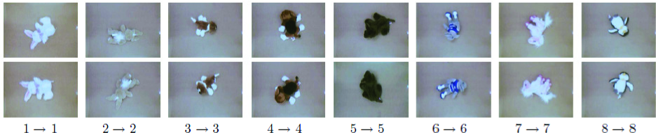
Results from matching query images obtained during a second run of the system (top) with images gathered during the first run (bottom). The numbers indicate the ground truth identity and the matched identity of the object.
The confusion matrix is shown in Table I, indicating the probability (according to the color histogram intersection) of each query image matching each database image. The higher the value, the more likely the two images match. Bold is used to indicate, for each query image, the database image that exceeds the Thmin threshold. In addition, recalling the classification threshold of Thmin described in section IV-A, each of the matches is considered valid except for #6, which is 0.01% below the threshold. As a result, this item would be incorrectly labeled as one that had not previously been seen.
Evaluating probabilities of soft toy animals: the rows represent query images and the columns represent database images.

In the cases of #1 and #7, the query image matched to two separate database images. In order to decide which query image was correctly related to a database image, the number of revolute joints were calculated. For each query image, the corresponding database image contained a higher number of revolute joints than the other database image, which clearly decided the correct objects to be matched. If the probability values were the only form of classification, then query image #1 would be misclassified. In this case, the skeleton was needed to properly classify the object.
D. Classification of metal and plastic recyclables
A practical example where the proposed approach could be particularly useful is that of separating items to be recycled from a pile of metal and/or plastic objects which are often thrown into a container without any organization. This experiment tests the ability of the system to locate small objects within a pile and be able to extract them for sorting, as in a recycling plant. We used bottles and cans which are representative types of the objects that may be found within a recycling container. The algorithm was able to distinguish between each item for extraction until all of the objects had been removed. After the item was extracted and classified, a sorting algorithm could be used to decide in which bin the object should be placed. Note that after the objects have been set aside for individual examination, it is much easier to determine their characteristics for such a sorting procedure than when they are cluttered in the entire group. The results of the experiment are shown in Figures 17, 18, and 19.
Example of a recycling experiment containing a pile of five plastic and metal objects that were individually separated and examined.
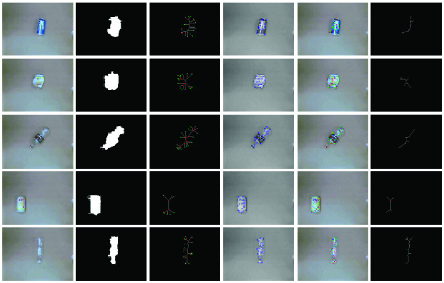
From left to right: The image taken after the object was isolated, the binary mask of the isolated object, the skeleton with the intersection points and end points labeled, the feature points gathered from the isolated object, the image after mapping the feature points to the intersections points, and the final skeleton with revolute joints labeled. Time flows from top to bottom, showing the progress as each individual object is examined.

Results from matching query images obtained during a second run of the system (top) with database images gathered during the first run (bottom) for the recycling experiment.
Due to the limitations of our current gripper, whenever the algorithm computed a grasp location, a human manually grasped the object at that location using an “EZ Reacher”, which is an aluminum pole with a handle that, when squeezed, causes two rubber cups at the other end to close, enabling extended grasping. While the human was grasping and moving the object, the algorithm continued to run as if a robot were in the loop. As a result, no modification to the algorithm was made.
The confusion matrix regarding the recycling experiment is in Table II, indicating the probability of each query image matching each database image. All of the cases, except for query image #1, were involved with having 2 query images match containing a probability value higher than Thmin. The deciding factor for grouping the correct images together was finding the revolute joints for each object. For each query image, the corresponding database image contained a higher number of revolute joints than the other database image, which clearly decided the correct objects to be matched, as in the previous experiment.
Evaluating probabilities of metal nad plastic: the rows represent query images and the columns represent database images.

E. Sorting of socks and shoes
Another practical example where the proposed approach would be particularly useful is that of sorting socks in a pile of laundry or organizing your shoes by grouping them with the corresponding pair. This experiment also tests the ability of the system to locate objects within a pile and to extract them for sorting as in the previous experiment. We used socks and shoes of different color and size to represent what you may see in a pile of laundry or shoes lying on the floor. The algorithm was able to distinguish between each item for extraction until all of the objects had been removed.
After the item was extracted and classified, a sorting algorithm could be used to decide whether the other half of the sock or shoe has been located or not. If the other half of the sock or shoe has not been examined previously, then that object is set aside until the other half has been extracted. Note that after the objects have been set aside for individual examination, it is much easier to determine their characteristics for such a matching procedure than when they are cluttered in the entire group. The results of the experiment are shown in Figures 20, 21, and 22.

Example of a service robot experiment containing a pile of socks and shoes that were individually separated and examined.
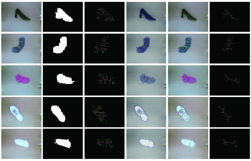
Example of a service robot experiment containing a pile of socks and shoes that were individually separated and examined. From left to right: The image taken after the object has been picked up and separated, the binary mask of the isolated object, the skeleton with the intersection points and end points labeled, the feature points gathered from the isolated object, the image after mapping the feature points to the intersections points, and the final skeleton with revolute joints labeled. Time flows from top to bottom, showing the progress as each individual object is examined.
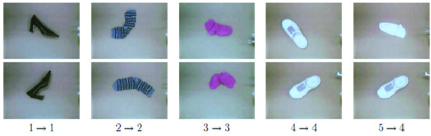
Results from matching query images obtained during a second run of the system (top) with database images gathered during the first run (bottom) for the recycling experiment.
Due to the limitations of our current gripper, the same steps were taken as in the previous experiment where the human manually grasped the object at a location using an “EZ Reacher”. While the human was grasping and moving the object, the algorithm continued to run as if a robot were in the loop. As a result, no modification to the algorithm was made.
The confusion matrix regarding the socks and shoes experiment is in Table III, indicating the probability of each query image matching each database image. All of the cases, except for query image #5, were correctly matched with the corresponding database image. In case #5, the white shoe and white sock were paired to be a match and resulted in an incorrect pairing. If the probability of query image #5 and database image #5 was higher than Thmin, then the white sock would have been correctly paired with the other white sock due to the number of revolute joints found through interaction. This experiment is an example of how two different objects can be mistakenly paired together through vision only.
Evaluating probabilities of socks and shoes: the rows represent query images and the columns represent database images

As a final experiment, to demonstrate that our approach works on articulated rigid objects, Figure 23 shows the original and final image along with the steps in achieving the end results for a pair of pliers. By comparing with Figure 6 of [11], it is clear that our approach extends that research by also including the ability to handle non-rigid objects.

Comparison of our approach to that of [11]. From top left to bottom right: The image taken after the object has been isolated, the binary mask of the isolated object, the skeleton with the intersection points and end points labeled, the feature points gathered from the isolated object, the image after mapping the feature points to the intersection points, and the final skeleton with revolute joints labeled.
6. Conclusion
We have proposed an approach to interactive perception in which a pile of unknown objects is sifted by an autonomous robot system in order to classify and label each item. The proposed approach has been found to be effective over a wide range of environmental conditions. The algorithm is shown empirically to provide a way to extract items out of a cluttered area one at a time with minimal disturbance to the other objects. This system uses a stereo camera system to identify the closest item in the scene. The information gathered from a single camera is sufficient to segment the various items within the scene and calculate a location for the robotic arm to grasp the next object for extraction. The stereo system is only used to calculate depth.
Monitoring the interaction of the object builds upon the approach in [11] to group different feature points together that share the same characteristics. The work in [11] also determined locations of revolute joints for planar rigid objects. Extending their work, the items that were monitored in our experiments were both rigid and non-rigid. This system demonstrates promising results for extraction and classification for cluttered environments.
The proposed approach only begins to address the challenging problem of interactive perception in cluttered environments. Other avenues can be explored in regards to improving the classification algorithm and learning strategy. When looking for a target item, one must consider the orientation of the object along with the angle from which it is viewed. Additional interaction and labeling techniques could be used to improve the ability of the system to determine which characteristics of an object make it distinguishable from other objects. Another improvement would be to incorporate a 3D model of the object instead of a 2D model.
Footnotes
7. Acknowledgements
This research was supported by the U.S. National Science Foundation under grants IIS-1017007, and IIS-0904116.