An Adaptive Three-Dimensional Nonlinear Path following Method for a Fix-Wing Micro Aerial Vehicle

Abstract

This paper describes an adaptive control approach of three-dimensional (3D) nonlinear path following for a fix-wing micro aerial vehicle (MAV) with wind disturbances in complicated terrain. We derive the control laws of course and flight path angle by the constructed Lyapunov function applying vector field theory based on the error equations in the Serret-Frenet frame, which are built by virtue of the relationship between the nonlinear desired trajectory and MAV. The 3D desired trajectory is fitted by using the fifth-order B-splines method through a sequence of waypoints created and sent by the ground station. Furthermore, the control laws are proved to be converged asymptotically and stably based on Lyapunov stability arguments. The results of the flight test experiment show that the flight could perform well under wind disturbances with a good trajectory tracking precision and high flight quality.

1. Introduction

Consisting of such advantages as limited volume, low mass, reasonable cost and rapid transportation, Micro-Aerial-Vehicles (MAVs) have demonstrated successful application in the military and civilian fields [1–5]. Furthermore, the path following problem of how to devise a simple real-time guidance law has proved to be quite challenging and has been a hot topic of research for many years as the problem will cause an ideal vehicle to converge at a defined path [6]. In practice, formation flying, target interception, border patrol are potential applications of MAVs, as well as convoy protection and air traffic holding patterns [7–10].

For MAVs, the wind disturbances, dynamic characteristics, the quality of sensing and control all limit the achievable tracking precision. As we know, primarily, wind speed is commonly 20–60 percent of the desired airspeed [11]. The effect deriving from this disturbance must be resolved by effective path tracking strategies. Then, for most fixed-wing MAVs, the minimum turn radius is in the range of 10–50 m, which produces a primary constraint on the spatial frequency of desired paths. Meanwhile, the high-resolution state sensors with high-frequency updates cannot be typically applied in MAVs. Thus, it is significant for research on the path tracking algorithms to improve the tracking precision, especially for MAVs.

Generally, people used MAVs in aerial photography and investigation, which require steady path following of a straight-line segment [11–13]. However, in complicated flight terrain, nonlinear path following would be required to perform special tasks and improve the flying quality. Before executing the flight missions, the nonlinear path is usually created by a sequence of waypoints which are uploaded from the ground station. To smooth the trajectory, the fitting method should be adapted. Furthermore, this method should also consider kinematic constraints on the MAV motion, expressed as upper bounds on the absolute values of velocity, acceleration and angular velocity. In [14] they fitted the waypoints into a smooth trajectory by fifth-order B-splines and also achieved good results in simulation with an optimal path following for the robot. In this paper, the fifth-order B-splines scheme is utilized in the overall nonlinear trajectory because of its simplicity and reliability in practice. The actual trajectories consist of a straight-line segment, an arc segment and other nonlinear segments. According to the criterion of the minimum energy and minimum manoeuvring, Zhu implemented the lateral path following based on the PID feedback method in simulation [8]. Baker achieved the path following using the PID control method based on a trajectory of coastline from a visual sensor [15]. Practically, the disturbances of the wind field affected to a fair extent the tracking precision for the MAVs. However, the paths of the straight-line segment and arc segment based on the vector field still could be tracked successfully, and their stability and convergence have been proved by Lyapunov functions [6, 11, 16]. In some special applications, other nonlinear paths, except for the arc segment, need to be analysed. Nonlinear path following with global asymptotic stability based on the dynamic model for ground-based robots also accomplished good results in simulation [17].

In the flight for MAVs, the velocity, angular rate and acceleration are continuously changing, thus it is important to fit and smooth the waypoints to improve the accuracy and quality of flight tracking. Firstly, the 3Dnonlinear path is designed by a sequence of waypoints applying the fifth-order B-splines method. Secondly, the error kinematic model for MAV is constructed by the position relationship between the nonlinear path and MAV. Then adaptive control laws for the course and flight path angle with anti-constant wind is established to ensure the global asymptotic stability of nonlinear tracking errors. Finally, the flight tests experiments have shown the effectiveness of the proposed method.

2. 3 D Nonlinear trajectory fitting

In typical applications, the flight trajectories are determined by a sequence of waypoints from the ground station. In order to generate smooth trajectories which can be effectively computed and memorized in real-time by the micro navigation computer in an MAV, the spline-functions are usually involved [14]. In this paper, the 3D trajectories with parameters, including continuous velocity, acceleration and derivative of acceleration, are designed by using the fifth-order B-splines. Therefore, the results of the first-order to third-order derivatives of trajectories are the continuous desired velocity, acceleration and derivative of the acceleration. The 3D trajectory is demonstrated as

$\{\begin{array}{l}x(s)={\displaystyle \sum _{j=0}^{n+4}{c}_{x_j}{\mathrm{\Omega }}_5(\frac{s-s_{j-2}}{h})}\\ y(s)={\displaystyle \sum _{j=0}^{n+4}{c}_{y_j}{\mathrm{\Omega }}_5(\frac{s-s_{j-2}}{h})}\\ z(s)={\displaystyle \sum _{j=0}^{n+4}{c}_{z_j}{\mathrm{\Omega }}_5(\frac{s-s_{j-2}}{h})}\end{array},$

(1)

where Ω₅ is the basic function of the fifth-order B-splines, n is the number of waypoints, s (a ≤ s ≤ b) is the arc length and (c_xj,c_yj,c_zj) is the control point.

In order to verify the effectiveness of the fifth-order B-splines' fitting method, a trajectory with solid-line in Fig.1 is fitted by a sequence of 21 waypoints. From Fig.1 we know that the circles are waypoints and the stars are control points. Fig.2 shows the results of first-order to third-order derivatives of 3D trajectory. From above, the solid lines are the derivative results of x(s), the dash-dot lines are the derivative results of y(s) and the dashed lines are the derivative results of z(s), the trajectories show continuous kinematic characteristics, which improve the flight trajectory tracking precision and flight quality.

Figure 1.

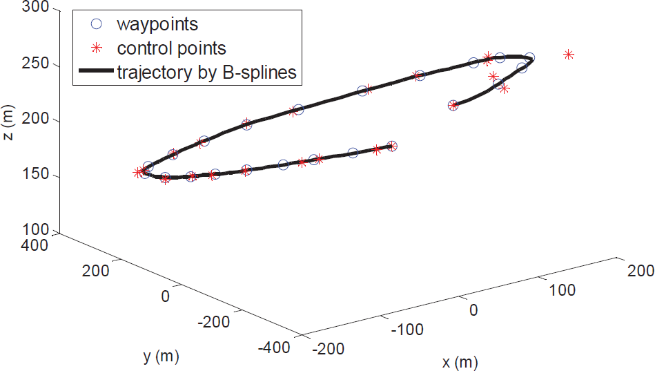
The 3D trajectory fitted by a fifth-order B-splines method

Figure 2.

The first-order to third-order derivatives of 3D trajectory

3. 3 D Trajectory error modelling

In this paper, the high frequency outputs of position [x y z] ^T , ground velocity V_g, flight path angle γ and the course χ can be calculated by the navigation computer based on the IMU (Inertial Measurement Unit) and GPS (Global Position System) for an MAV. Simultaneously, the airspeed V_a can be monitored by pressure sensors. Usually, the control laws of course and flight path angle with the assumption of a constant wind disturbance W = [W_x W_y W_z] ^T can be designed, so that the flight trajectory could accurately approach the desired trajectory. Therefore, the kinematics equations extended by [11] are defined as

$\{\begin{array}{l}\dot{x}=V_a\cos \psi \cos \gamma +W_x=V_g\cos \chi \cos \gamma \\ \dot{y}=V_a\sin \psi \cos \gamma +W_y=V_g\sin \chi \cos \gamma \\ \dot{z}=-V_a\sin \gamma +W_z=-V_g\sin \gamma \\ \dot{\chi }=\alpha ({\chi }_c-\chi )\\ \dot{\gamma }=\beta ({\gamma }_c-\gamma )\end{array},$

(2)

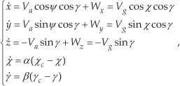
where Ψ is the carrier heading, χ _c is the target course, γ_c is the target flight path angle, α is the response coefficient of course and β is the response coefficient of flight path angle.

The Geometric graph among the MAV, desired trajectory and inertial frame is shown in Fig.3. We know that the distance vector of the vehicle's centre of gravity Q in the inertial frame {I} can be expressed by, the distance vector of the tracking point P on the desired path in {I} can be denoted by in Serret-Frenet frame {F}, the distance vector between the P and Q in {I} is in {F}, the {B} is the body frame for MAV, is the trajectory tangent angle, is the trajectory velocity of P and is the tangent direction coordinate of P in {F}.

Figure 3.

Geometric graph among MAV, desired trajectory and inertial frame

Let

$\begin{array}{l}R=C_I^F({\chi }_f,{\gamma }_f)={\left[C_F^I({\chi }_f)\right]}^T\\ =\left(\begin{array}{ccc}\cos ({\gamma }_f)& 0& -\sin ({\gamma }_f)\\ 0& 1& 0\\ \sin ({\gamma }_f)& 0& \cos ({\gamma }_f)\end{array}\right)\left(\begin{array}{ccc}\cos ({\chi }_f)& \sin ({\chi }_f)& 0\\ -\sin ({\chi }_f)& \cos ({\chi }_f)& 0\\ 0& 0& 1\end{array}\right)\\ =\left(\begin{array}{ccc}\cos ({\gamma }_f)\cos ({\chi }_f)& \cos ({\gamma }_f)\sin ({\chi }_f)& -\sin ({\gamma }_f)\\ -\sin ({\chi }_f)& \cos ({\chi }_f)& 0\\ \sin ({\gamma }_f)\cos ({\chi }_f)& \sin ({\gamma }_f)\sin ({\chi }_f)& \cos ({\gamma }_f)\end{array}\right)\end{array}$

(3)

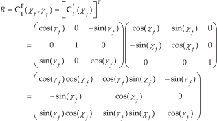
be the rotation matrix from {I} to {F}, parameterized locally by the angles χ_f and χ_f. Then the angular velocity on P can be expressed in {I} to yield

${\omega }_F=\left[\begin{array}{l}0\\ {\dot{\gamma }}_f\\ 0\end{array}\right]+\left(\begin{array}{ccc}\cos ({\gamma }_f)& 0& -\sin ({\gamma }_f)\\ 0& 1& 0\\ \sin ({\gamma }_f)& 0& \cos ({\gamma }_f)\end{array}\right)\left[\begin{array}{l}0\\ 0\\ {\dot{\chi }}_f\end{array}\right]=\left[\begin{array}{l}-{\dot{\chi }}_f\sin ({\gamma }_f)\\ {\dot{\gamma }}_f\\ {\dot{\chi }}_f\cos ({\gamma }_f)\end{array}\right],$

(4)

where the values of ${\dot{\gamma }}_f$ and ${\dot{\chi }}_f$ can be computed as

$\{\begin{array}{l}{\dot{\chi }}_f=\frac{d{\chi }_f}{ds}\frac{ds}{dt}=\frac{d{\tan }^{-1}({y^{\prime }}_f/{x^{\prime }}_f)}{ds}\dot{s}=\frac{{x^{\prime }}_f{y^{″}}_f-{x^{″}}_f{y^{\prime }}_f}{{({x^{\prime }}_f{}^2+{y^{\prime }}_f{}^2)}^{3/2}}\dot{s}=\tau (s)\dot{s}\\ {\dot{\gamma }}_f=\frac{d{\gamma }_f}{ds}\frac{ds}{dt}=\frac{d{\tan }^{-1}({z^{\prime }}_f/\sqrt{{y^{\prime }}_f{}^2+{x^{\prime }}_f{}^2})}{ds}\dot{s}=\\ =\frac{{z^{″}}_f\left({y^{\prime }}_f{}^2+{x^{\prime }}_f{}^2\right)-{z^{\prime }}_f\left({y^{\prime }}_f{y^{″}}_f+{x^{\prime }}_f{x^{″}}_f\right)}{\sqrt{{y^{\prime }}_f{}^2+{x^{\prime }}_f{}^2}\left({y^{\prime }}_f{}^2+{x^{\prime }}_f{}^2+{z^{\prime }}_f{}^2\right)}\dot{s}=\varsigma (s)\dot{s}\end{array},$

(5)

where τ(s) and ς(s) denote the path curvature. The velocity of P in {I} can be expressed in {F} to yield

${\left(\frac{dp}{dt}\right)}_F={\left[\begin{array}{ccc}\dot{s}& 0& 0\end{array}\right]}^T.$

(6)

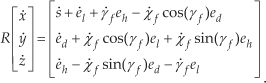
It is also straightforward to compute the velocity of Q in {I} as

${\left(\frac{dq}{dt}\right)}_I={\left(\frac{dp}{dt}\right)}_I+R^{-1}{\left(\frac{de}{dt}\right)}_F+R^{-1}\left({\omega }_F\times e\right).$

(7)

Multiplying the above equation on the left by R gives the velocity of Q in {I} expressed in {F} as

$R{\left(\frac{dq}{dt}\right)}_I={\left(\frac{dp}{dt}\right)}_F+{\left(\frac{dr}{dt}\right)}_F+\left({\omega }_F\times e\right).$

(8)

Using the relations

${\left(\frac{dq}{dt}\right)}_I={\left[\begin{array}{ccc}\dot{x}& \dot{y}& \dot{z}\end{array}\right]}^T,\hspace{0.17em}\hspace{0.17em}{\left(\frac{de}{dt}\right)}_F={\left[\begin{array}{ccc}{e}_l& e_d& e_h\end{array}\right]}^T,$

and

$\left({\omega }_F\times e\right)=\left[\begin{array}{l}-{\dot{\chi }}_f\sin ({\gamma }_f)\\ {\dot{\gamma }}_f\\ {\dot{\chi }}_f\cos ({\gamma }_f)\end{array}\right]\times \left[\begin{array}{l}{e}_l\\ e_d\\ e_h\end{array}\right]=\left[\begin{array}{l}{\dot{\gamma }}_f{e}_h-{\dot{\chi }}_f\cos ({\gamma }_f)e_d\\ {\dot{\chi }}_f\cos ({\gamma }_f)e_l+{\dot{\chi }}_f\sin ({\gamma }_f)e_h\\ -{\dot{\chi }}_f\sin ({\gamma }_f)e_d-{\dot{\gamma }}_f{e}_l\end{array}\right].$

Eq. (8) can be rewritten as

$R\left[\begin{array}{l}\dot{x}\\ \dot{y}\\ \dot{z}\end{array}\right]=\left[\begin{array}{l}\dot{s}+{\dot{e}}_l+{\dot{\gamma }}_f{e}_h-{\dot{\chi }}_f\cos ({\gamma }_f)e_d\\ {\dot{e}}_d+{\dot{\chi }}_f\cos ({\gamma }_f)e_l+{\dot{\chi }}_f\sin ({\gamma }_f)e_h\\ {\dot{e}}_h-{\dot{\chi }}_f\sin ({\gamma }_f)e_d-{\dot{\gamma }}_f{e}_l\end{array}\right].$

Solving for ė_l, ė_d and ė_h yields

$\{\begin{array}{l}{\dot{e}}_l=V_g\cos (\gamma -{\gamma }_f)\cos (\chi -{\chi }_f)-\dot{s}-{\dot{\gamma }}_f{e}_h+{\dot{\chi }}_f\cos ({\gamma }_f)e_d\\ {\dot{e}}_d=V_g\cos (\gamma -{\gamma }_f)\sin (\chi -{\chi }_f)-{\dot{\chi }}_f\cos ({\gamma }_f)e_l-{\dot{\chi }}_f\sin ({\gamma }_f)e_h\\ {\dot{e}}_h=-V_g\sin (\gamma -{\gamma }_f)-{\dot{\chi }}_f\sin ({\gamma }_f)e_d-{\dot{\gamma }}_f{e}_l\end{array}.$

(9)

Finally from Eq. (2) and (9), the trajectory error kinematic model can be expressed as

$\{\begin{array}{l}{\dot{e}}_l=V_g\cos (\tilde{\gamma })\cos (\tilde{\chi })-\dot{s}-{\dot{\gamma }}_f{e}_h+{\dot{\chi }}_f\cos ({\gamma }_f)e_d\\ {\dot{e}}_d=V_g\cos (\tilde{\gamma })\sin (\tilde{\chi })-{\dot{\chi }}_f\cos ({\gamma }_f)e_l-{\dot{\chi }}_f\sin ({\gamma }_f)e_h\\ {\dot{e}}_h=-V_g\sin (\tilde{\gamma })-{\dot{\chi }}_f\sin ({\gamma }_f)e_d-{\dot{\gamma }}_f{e}_l\\ \dot{\stackrel{~}{\chi }}=\alpha ({\chi }_c-\chi )+{\dot{\chi }}_f\\ \dot{\stackrel{~}{\gamma }}=\beta ({\gamma }_c-\gamma )+{\dot{\gamma }}_f\end{array}.$

(10)

We can conclude that the tracking problem can be substituted by the problem that the errors in the formula (10) tend to zero. According to the error equations, in the nonlinear path following process, if the ground speed V_g, position (x,y,z), course χ, desired course χ_f, flight path angle γ, desired flight path angle γ _f , forward error e_l, lateral error e_d and longitude error e_h are determined, the target course χ _c and flight path angle γ _c can be calculated.

4. Adaptive Control Laws

In order to achieve nonlinear trajectory tracking, the control laws of course χ _c and flight path angle γ _c are designed to make the errors tend to zero according to the formula (10). From the distance errors of e_d and e_h, and the vector field theory [11], the desired course error and flight path angle error are assumed as

$\{\begin{array}{l}{\chi }_d(e_d)=-{\chi }_{\infty }\frac{2}{\pi }{\tan }^{-1}(k{e}_d)\\ {\gamma }_h(e_h)={\gamma }_{\infty }\frac{2}{\pi }{\tan }^{-1}(m{e}_h)\end{array},$

(11)

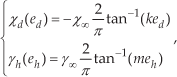
where χ _∞ ∈ (0,π/2] and γ_∞ ∈ (0,π/2] are maximums of desired course error and desired flight path angle error with absolute value when e_d and e_h is the infinity respectively, k > 0 and m > 0 are the coefficients about the dynamic characteristic for an MAV.

From formula (11) we will obtain that when e_d → 0 then χ_d(e_d) → 0 and e_h → 0 then γ _h (e_h) → 0. Thereby, -e_d sin(χ _d (e_d)) ≥ 0 and e_h sin(γ _h (e_h)) ≥ 0, for e_d,e_h ∈ R are obviously satisfied.

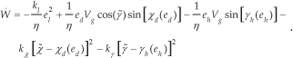
From above, the Lyapunov function can be constructed from formulae (10) and (11) as follows

$W=\frac{1}{2\eta }(e_d^2+e_l^2+e_h^2)+\frac{1}{2}{\left[\tilde{\chi }-{\chi }_d(e_d)\right]}^2+\frac{1}{2}{\left[\tilde{\gamma }-{\gamma }_h(e_h)\right]}^2,$

(12)

where, the first item of Lyapunov function is to make the distance error between the MAV and the desired trajectory tend to zero; the second item is to satisfy desired course error as close as possible, and the third item is to bring desired flight path angle error as close as possible.

Furthermore, the time derivative of W results in

$\begin{array}{l}\dot{W}=\frac{1}{\eta }({\dot{e}}_l{e}_l+{\dot{e}}_d{e}_d+{\dot{e}}_h{e}_h)+\left[\tilde{\chi }-{\chi }_d(e_d)\right]\left[\dot{\stackrel{~}{\chi }}-{\dot{\chi }}_d(e_d)\right]+\left[\tilde{\gamma }-{\gamma }_h(e_h)\right]\left[\dot{\stackrel{~}{\gamma }}-{\dot{\gamma }}_h(e_h)\right]=\\ \frac{1}{\eta }\left\{\begin{array}{l}{e}_l\left[V_g\cos (\tilde{\gamma })\cos (\tilde{\chi })-\dot{s}-\varsigma (s)\dot{s}{e}_h+\tau (s)\dot{s}\cos ({\gamma }_f)e_d\right]+\\ e_d\left[V_g\cos (\tilde{\gamma })\sin (\tilde{\chi })-\tau (s)\dot{s}\cos ({\gamma }_f)e_l-\tau (s)\dot{s}\sin ({\gamma }_f)e_h\right]+\\ e_h\left[-V_g\sin (\tilde{\gamma })+\tau (s)\dot{s}\sin ({\gamma }_f)e_d+\varsigma (s)\dot{s}{e}_l\right]\end{array}\right\}+\\ \left[\tilde{\chi }-{\chi }_d(e_d)\right]\left\{\begin{array}{l}\alpha ({\chi }_c-\chi )-\tau (s)\dot{s}-{{\chi }^{\prime }}_d(e_d)\\ \left[V_g\cos (\tilde{\gamma })\sin (\tilde{\chi })-\tau (s)\dot{s}\cos ({\gamma }_f)e_l-\tau (s)\dot{s}\sin ({\gamma }_f)e_h\right]\end{array}\right\}+\\ \left[\tilde{\gamma }-{\gamma }_h(e_h)\right]\left\{\begin{array}{l}\beta ({\gamma }_c-\gamma )-\varsigma (s)\dot{s}-{\gamma }_h^{\text{'}}(e_h)\\ \left[-V_g\sin (\tilde{\gamma })+\tau (s)\dot{s}\sin ({\gamma }_f)e_d+\varsigma (s)\dot{s}{e}_l\right]\end{array}\right\},\end{array}$

and then

$\begin{array}{l}\dot{W}=\frac{1}{\eta }{e}_l\left[V_g\cos (\tilde{\gamma })\cos (\tilde{\chi })-\dot{s}\right]+\frac{1}{\eta }{e}_d{V}_g\cos (\tilde{\gamma })\sin \left[{\chi }_d(e_d)\right]-\\ \hspace{0.17em}\hspace{0.17em}\hspace{0.17em}\hspace{0.17em}\hspace{0.17em}-\frac{1}{\eta }{e}_h{V}_g\sin \left[{\gamma }_h(e_h)\right]\hspace{0.17em}+\left[\tilde{\chi }-{\chi }_d(e_d)\right]\\ \left\{\begin{array}{l}\alpha ({\chi }_c-\chi )-\tau (s)\dot{s}-{{\chi }^{\prime }}_d(e_d)\left[V_g\cos (\tilde{\gamma })\sin (\tilde{\chi })-\tau (s)\dot{s}\cos ({\gamma }_f)e_l-\tau (s)\dot{s}\sin ({\gamma }_f)e_h\right]+\\ \frac{e_d{V}_g\cos (\tilde{\gamma })\left[\sin (\tilde{\chi })-\sin ({\chi }_d(e_d)\right]}{\eta \left[\tilde{\chi }-{\chi }_d(e_d)\right]}\end{array}\right\}+\\ \left[\tilde{\gamma }-{\gamma }_h(e_h)\right]\left\{\begin{array}{l}\beta ({\gamma }_c-\gamma )-\varsigma (s)\dot{s}-{\gamma }_h^{\text{'}}(e_h)\left[-V_g\sin (\tilde{\gamma })+\tau (s)\dot{s}\sin ({\gamma }_f)e_d+\varsigma (s)\dot{s}{e}_l\right]+\\ \frac{e_h{V}_g\left[-\sin (\tilde{\gamma })+\sin ({\gamma }_h(e_h)\right]}{\eta \left[\tilde{\gamma }-{\gamma }_h(e_h)\right]}\end{array}\right\}\end{array}$

(13)

Therefore, the control laws can be designed as follows

$\begin{array}{l}{\chi }_c=k_{\chi }\left[\tilde{\chi }-{\chi }_d(e_d)\right]+\chi +\frac{1}{\alpha }\tau (s)\dot{s}+\\ \frac{1}{\alpha }{{\chi }^{\prime }}_d(e_d)\left[V_g\cos (\tilde{\gamma })\sin (\tilde{\chi })-\tau (s)\dot{s}\cos ({\gamma }_f)e_l-\tau (s)\dot{s}\sin ({\gamma }_f)e_h\right]-\\ \frac{1}{\alpha } \frac{e_d{V}_g\cos (\tilde{\gamma })\left[\sin (\tilde{\chi })-\sin ({\chi }_d(e_d)\right]}{\eta \left[\tilde{\chi }-{\chi }_d(e_d)\right]}\\ {\gamma }_c=k_{\gamma }\left[\tilde{\gamma }-{\gamma }_h(e_h)\right]+\gamma +\frac{1}{\beta }\varsigma (s)\dot{s}+\\ \frac{1}{\beta }{\gamma }_h^{\text{'}}(e_h)\left[-V_g\sin (\tilde{\gamma })+\tau (s)\dot{s}\sin ({\gamma }_f)e_d+\varsigma (s)\dot{s}{e}_l\right]-\\ \frac{1}{\beta }\frac{e_h{V}_g\left[-\sin (\tilde{\gamma })+\sin ({\gamma }_h(e_h))\right]}{\eta \left[\tilde{\gamma }-{\gamma }_h(e_h)\right]}\\ \dot{s}=k_l{e}_l+V_g\cos (\tilde{\gamma })\cos (\tilde{\chi }),\end{array}$

(14)

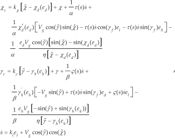
where k_χ, k_γ, k_l and η are the coefficients which make the state variables $\tilde{\chi },\hspace{0.17em}\tilde{\gamma },\hspace{0.17em}{e}_l,\hspace{0.17em}{e}_d$ and e_h tend to zero, respectively.

In order to validate the stability of the control laws of course and flight path angle, taking formula (14) into formula (13), we can obtain as follows

$\begin{array}{l}\dot{W}=-\frac{k_l}{\eta }{e}_l^2+\frac{1}{\eta }{e}_d{V}_g\cos (\tilde{\gamma })\sin \left[{\chi }_d(e_d)\right]-\frac{1}{\eta }{e}_h{V}_g\sin \left[{\gamma }_h(e_h)\right]-\\ k_{\chi }{\left[\tilde{\chi }-{\chi }_d(e_d)\right]}^2-k_{\gamma }{\left[\tilde{\gamma }-{\gamma }_h(e_h)\right]}^2.\end{array}$

(15)

From the above equation, if only e_d = e_l = e_h = 0, χ_d = χ_f, and γ_h = γ_f then Ẇ = 0, and if otherwise, then Ẇ < 0. According to the Lyapunov stability theorem, the $\underset{t\to \infty }{\lim }{e}_d=0,\hspace{0.17em}\underset{t\to \infty }{\lim }{e}_l=0,\hspace{0.17em}\underset{t\to \infty }{\lim }{e}_h=0,\hspace{0.17em}\underset{t\to \infty }{\lim }\tilde{\chi }={\chi }_d(e_d)\to 0$ , and $\underset{t\to \infty }{\lim }\tilde{\gamma }={\gamma }_h(e_h)\to 0$ . Therefore, the control laws designed in this paper are global asymptotic stability.

5. Special trajectory analysis – straight-line segments in 3D space

As we know, the straight-line segments in space for 3D path following can be defined by formula (1)

$\{\begin{array}{l}x=x_0+s\cos \lambda \cos \rho \\ y=y_0+s\cos \lambda \sin \rho \\ z=z_0-s\sin \lambda \end{array}.$

(16)

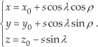
where (x₀,y₀,z₀) is the starting point; λ and ρ is the flight path angle and course for the straight line respectively.

With formulae (5) and (16), we can get

$\{\begin{array}{l}{\chi }_f=\rho \\ {\dot{\chi }}_f=\tau (s)\dot{s}=0\\ {\gamma }_f=\lambda \\ {\dot{\gamma }}_f=\varsigma (s)\dot{s}=0\end{array}.$

(17)

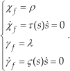
Finally, the control laws of course and flight path angle for straight path following in 3D space are derived as

$\begin{array}{l}{\chi }_c=k_{\chi }\left[\tilde{\chi }-{\chi }_d(e_d)\right]+\chi +\frac{1}{\alpha }{{\chi }^{\prime }}_d(e_d)V_g\cos (\tilde{\gamma })\sin (\tilde{\chi })-\\ \frac{1}{\alpha } \frac{e_d{V}_g\cos (\tilde{\gamma })\left[\sin (\tilde{\chi })-\sin ({\chi }_d(e_d)\right]}{\eta \left[\tilde{\chi }-{\chi }_d(e_d)\right]}\\ {\gamma }_c=k_{\gamma }\left[\tilde{\gamma }-{\gamma }_h(e_h)\right]+\gamma -\\ \frac{1}{\beta }{\dot{\gamma }}_h(e_h)V_g\sin (\tilde{\gamma })-\\ \frac{1}{\beta }\frac{e_h{V}_g\left[-\sin (\tilde{\gamma })+\sin ({\gamma }_h(e_h)\right]}{\eta \left[\tilde{\gamma }-{\gamma }_h(e_h)\right]}\\ \dot{s}=k_l{e}_l+V_g\cos (\tilde{\gamma })\cos (\tilde{\chi }).\end{array}$

(18)

6. Results and analysis of flight tests

In this section, experimental results from implementing the proposed 3D nonlinear path following algorithm are discussed. First, the experimental system is briefly introduced and then the flight test results of 3D path following are presented.

6.1 Experimental system

The demonstration system is mainly composed of an MAV (the basic parameters are shown in Table 1) and an autopilot system (both of which are shown in Fig. 4). The autopilot system plays a vital role in the MAV system because it is in charge of raw data collection, which is carried out by an assemblage of diverse sensors. The sensor inputs consist of many parts as follows: gyroscopes (three axis), accelerometers (three axis), magnetometers (three axis), static and dynamic pressure, and miniature GPS receiver. The signal process hardware system mainly includes a digital signal processor (DSP) and a microcontroller. All the inertial devices and sensors are MEMS-based, while other hardware components are solid state. In addition, the DSP enables sophisticated algorithms of error compensation, strapdown and Kalman filter with 15 states [18], which is able to calculate the angular rates w, acceleration a, flight path angle γ, roll angle φ, position (x,y,z) and ground speed V_g. Similarly, with the results of DSP, the controller has the ability to implement complicated flight control functions including a fully autonomous flight controller. In practice, the operational precision measured by the sensors and estimated by the filters for an MAV also has an important effect on good-performance in the autonomous flight controller, whose benchmark is a highly accurate Position Orientation System (POS) [19]. The comparative results were summarized in Table 2.

Figure 4.

The MAV and autopilot

Table 1.

The basic parameters for the MAV

Fuselage length (m)	Wing span (m)	Chord length (m)	Takeoff weight (kg)	load (kg.m−2)	velocity (km.h−1)	Flight radius (km)
2.25	3.40	0.43	12.5	9.084	70∼120	30

Table 2.

The navigation measurement precision for the autopilot

γ (°)	φ (°)	‖ (x, y, z)‖ (m)	Vg (m/s)	χ (°)	w (°/s)	a (m/s2)
0.5507	0.4637	2.2985	0.3068	1.65	0.03	10e-3

The parameters in flight can be taken as k_l = 0.5, k_χ =0.005, k_γ =0.005, χ_∞ = π/2, γ_∞/4, k = 0.05, m = 0.05, α = 0.8, β = 0.8, η = 2000.

6.2 Flight test results for 3D path following

In this paper, the straight-line segments in space for 3D path following are employed to illuminate the tracing precision of the proposed method. The experimental results of flight trajectory with x-y-height are shown in Fig. 5 with solid-line segments and the dashed-line segments are the referenced paths. We can see that the starts of No.1(-1000, 1000, 500), No.2 (1000,1000, 500), No.3(1000,-3000, 500) and No.4(-1000,-3000, 500) are cruising waypoints, and the starts of No.5 (50,700,450), No.6 (50,-150,410), No.7 (-150,-150,410), No.8 (-150,700,390), No.9 (50,700,390), No.10 (50,-150,340), No.11 (-150,-150,340), No.12 (-150,700,320), No.13 (50, 700, 320) and No.14 (50, 550, 310) are automatically descending waypoints.

Figure 5.

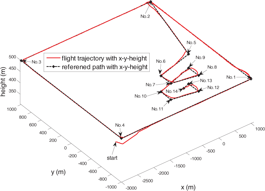
The 3D flight path

Fig. 5 shows that the flight path is basically consistent with the expected track, and in cruising state, the tracking precision has a standard deviation of 1.2 m. Since in the corner part of the flight path the MAV could not achieve the expected angle rate, besides, the goal roll angle is limited and the wingspan manoeuvrability of the MAV is long and poor, therefore the flight path could not be in accordance with the desired track and the overshoot appeared in flight. The state variables of χ, γ, φ, height h_p, airspeed V_a and V_g in flight process are in Fig. 6–11

Figure 6.

The course for 3D flight path

Figure 7.

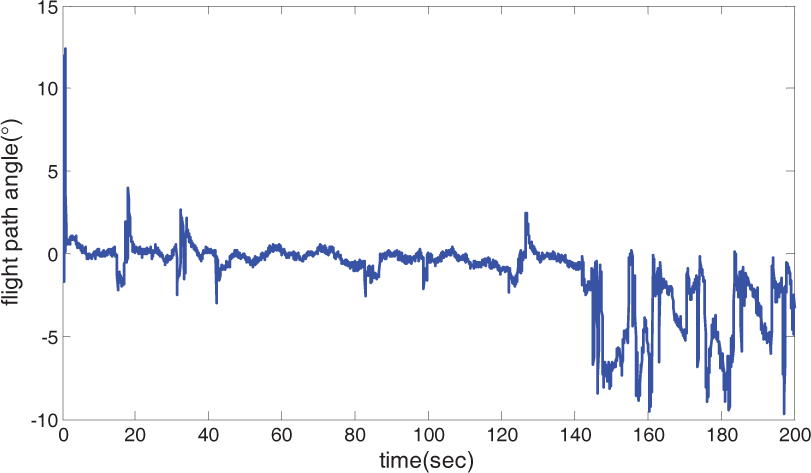
The flight path angle for 3D flight path

Figure 8.

The roll for 3D flight path

Figure 9.

The height for 3D flight path

Figure 10.

The airspeed for 3D flight path

Figure 11.

The ground velocity for 3D flight path

In Fig. 6, when the MAV follows the directions of north, west, south, east, the courses are holding at about 360, 270, 180, 90 degrees respectively. In Fig. 7, when the MAV is in the cruising state, the flight path angle keeps at about zero, and when the MAV is in the descending state, the flight path angle changes with the desired path. In Fig. 8, the max of φ is about 10 degrees in the turn state. In Fig. 9, the height almost maintains at 500 m in cruising state with a standard deviation of 1.5 m. In the experiment, the airspeed is controlled at a constant of about 30 m/s to keep the engine in a steady state shown in Fig. 10, and we can see that the airspeed is consistent with the target airspeed. Furthermore, from the ground speed in Fig.11 we can conclude that the wind speed is about 5.3 m/s in cruising state.

The 3D flight path has demonstrated that the proposed method has good repeatability and adaptability. Therefore, the results of flight experiments have proved that the proposed nonlinear adaptive flight path tracking control method is effective and practical.

7. Conclusion

In this paper, we have proposed a new approach for three-dimensional nonlinear path following based on the use of Lyapunov theory for MAVs. To the best of our knowledge, the designed adaptive control method is not dependent on the dynamic model of MAVs and can also be achieved in application with simple hardware. The algorithm can be applied to following the 3D smooth nonlinear trajectory, which is fitted by an arbitrary sequence of waypoints using the fifth-order B-splines method and is proved to have high flight quality. Finally, the flight experiment of 3D path following achieves the high trajectory tracking precision with standard deviations of 1.5 m in height direction and 1.2 in plane geometry respectively in the wind disturbances of 5.3 m/s.