Sage Journals: Discover world-class research

Abstract

This article concerns airflow-based odometry for estimating MAV flight speed from airflow measurements provided by a set of thermal anemometers. Our approach relies on a Gated Recurrent Unit (GRU) based deep learning approach to extract deep features from noisy and turbulent measurement signals of triaxial thermal anemometers, in order to establish the underlying mapping between the airflow measurement and the flight speed. The proposed solution is validated on a multi-rotor MAV. The results show that the GRU-based model can effectively extract noise features and perform denoising, and compensate for induced velocity effects along the propellers’ rotation axis. As a consequence, robust prediction of the flight speed is performed, including during takeoff and landing that induce ground effects and strong variations of vertical airflow.

Keywords

Thermal anemometer deep learning odometry multi-rotor Micro Aerial Vehicle(MAV)

SOURCE CODE

Our open source implementation and more details are available at https://github.com/SyRoCo-ISIR/Flight-Speed-Estimation-Airflow.git

Introduction

Estimation of the 3D velocity and/or position of a MAV is essential for both tele-operated and fully autonomous missions. Different sensing modalities can be used to this purpose, which can be roughly divided into three categories: External perception systems (UWB odometry, GPS,¹ Motion Capture system²), Exteroceptive sensors (Lidar odometry,³ visual odometry(VO)^4,5), and Proprioceptive sensors (inertial navigation system(INS)¹). Each category of sensors comes with its own advantages and drawbacks, especially in the context of MAV applications. External perception systems, when available, are very convenient as they require limited payload (both material and computational) aboard the drone, but they are not always available since the service is provided independently of the MAV. Exteroceptive sensors provide information about the MAV’s environment that is extremely useful for sense and avoid applications, but they often require heavy computational payload, and they are subjected to environmental conditions (illumination, visual texture, etc.). Proprioceptive sensors (INS, or odometry based on Blade Element and Momentum theory for multi-rotor MAVs⁶) use little embarked payload, are always available, and can provide good speed estimation over very short time-intervals, but they are subjected to drift when used for position estimation. Thus, there is no universal sensory modality but each one can be useful or even crucial in specific contexts, thus contributing to a global sensor-fusion architecture.

This paper concerns the problem of MAVs’ velocity/air-velocity estimation from measurements provided by thermal anemometers. Here, “air-velocity” denotes the MAV’s velocity relative to air. A thermal anemometer, as illustrated on Figure 1, is a cylindrical sensor that provides information about the airflow that passes through the device. It can thus be viewed as a 1D airspeed sensor. When used in still air (the typical indoor situation), it thus provides information about the sensor’s velocity along the cylinder’s axis. When used outdoor, it provides information about the sensor’s air-velocity along the cylinder’s axis, similar to a Pitot tube. Using a set of three orthogonal thermal anemometers to estimate the 3D velocity/air-velocity of a multi-rotor MAV, as illustrated by Figure 1, is not straightforward. The main difficulty comes from the airflow generated by the propellers, especially in the vertical direction (in body frame) where airflow velocity is the sum of the induced velocity and MAV’s velocity. In addition, as with any sensor, measurements are noisy, where noise may be electronic or “mechanical” (related, e.g., to vibrations aboard the MAV). By combining a simple analytical sensor model and a neural network architecture, we show that good speed estimates can be obtained in all flight phases, including take-off and landing. In particular, the neural network proves helpful in correcting induced velocity related biases in the (body relative) vertical direction and reducing “noise”. Concerning noise reduction, note that similar conclusions about the benefit of neural networks were drawn for attitude estimation based on IMU measurements.⁷ We investigated several different neural networks architectures such as LSTM, MLP, and WaveNet, and found that the GRU-based architecture performs best in estimating the flight speed.

Figure 1.

MAV equipped with three thermal anemometers orthogonal to each other.

This paper is an extension of the IMAV 2022 conference paper,⁸ which was one the papers selected for the best paper nomination. With respect to Wang et al.,⁸ the present article provides complements at two levels: first, we evaluate the odometry drift when integrating the obtained velocity estimates to produce displacement estimates; then, we provide complementary experimental validations with another sensor configuration and more aggressive flights to evaluate the robustness of the approach.

The paper is organized as follows. Section Airflow sensors for MAVs provides a literature review concerning the different types of airflow sensors in the context of MAVs applications. A simple model of the thermal anemometer measurement is proposed in Section Thermal Anemometer Measurement Model. Outputs of this model are then used as inputs of the deep learning-based architecture presented in Section Deep learning-based prediction with airflow. Experimental results obtained with the proposed method and the MAV of Figure 1 are reported in Section Implementation & Results. The paper ends with a conclusion and perspectives.

Airflow sensors for MAVs

There are many types of anemometers that rely on different measurement techniques, and they are usually divided into two categories: velocity anemometers, which directly convert airflow speed into other physical signals (such as Cup/Vane anemometers, Hot-wire anemometers based on Thermal Dissipation,^9–11 Laser anemometers based on Doppler shift, Ultrasonic anemometers based on ToF¹²), and dynamic pressure anemometers, which are able to sense the dynamic pressure of the air directly and then derive the airflow speed (such as Pitot-Tube anemometers based on Bernoulli’s principle,¹³ Hall sensor based anemometer according to the deflection angle under static equilibrium).

Recently, researchers have also designed custom-made sensors based on the above principles. Inspired by bionic ideas, a whisker-like sensor is presented in Prudden et al.,¹³ and combined with a barometer that acts as a force sensor to measure the airflow pressure signal coming from the whiskers. The idea of a bionic whisker is also employed in Tagliabue et al.¹⁴ to design a dedicated anemometer but Hall sensors are used to measure the displacement of magnetic objects caused by air drag. Another work that also uses Hall sensors is in Zahran et al.,¹⁵ but differently it leverages airflow pressure to push a pendulum-like plate, thus using Hall sensors to measure the deflection angle and thus predict the airflow speed. Other solutions based on converting the airflow information into a motion information include,^16,14,15 where both Tagliabue et al.¹⁴ and Zahran et al.¹⁵ use Hall sensors to directly capture the electrical signal from the motion, while¹⁶ converts it into a pressure variation on an embedded barometer. In comparison, the whisker-like structure has a smaller size and thus is more sensitive to the variation of airflow and thus has a higher resolution, while the plate structure has a larger measurement range and less turbulence effects. The work in Tagliabue et al.¹⁴ stands perfectly in-between: wide measuring range on the one hand and high resolution on the other hand. All these solutions rely on mechanical moving parts, however, which can be an issue in term of mechanical robustness and maintenance.

Solutions that do not require mechanical moving parts include laser Doppler anemometers, ultrasonic anemometers, thermal anemometers, and Pitot tubes. Laser Doppler anemometers are suitable for high precision scenarios but are not suited to MAVs due to their size and price. Pitot tubes are unidirectional and usually applied to fixed-wing aircraft. The TriSonica Mini ultrasound anemometer on Figure 2 was used in Hollenbeck et al.¹² Although being the most compact 2D ultrasound anemometer on the market, it is still heavy for MAV applications and expensive. The SFM3000 thermal anemometer on Figure 3 was used in both Li et al.¹¹ and Müller et al.¹⁰ It is a 1D bidirectional anemometer and weights only 17g, with a data output rate of 2kHz, a measurement range of 200 standard liters per minute (slm) and a resolution of $\pm 2.5$ %. This sensor was chosen for this work due to its numerous advantages: large flow range, high accuracy, high repeatability, high reliability, good linearity and sensitivity, and easy maintenance due to the absence of moving mechanical parts.

Figure 2.

TriSonica Mini Wind Sensor is the World’s smallest ( $91 \times 91 \times 52$ mm) and lightest (50 grams) low velocity (less than 50 m/s) ultrasonic anemometer with a maximum data output rate of 60 Hz.

Figure 3.

SFM3000 from Sensirion AG is a bi-directional hot-wire anemometer, which is compact ( $82 \times 35 \times 32$ mm), lightweight (17 grams) and high data output rate (up to 2 kHz).

Thermal anemometer measurement model

The measurement principle of the bi-directional thermal anemometer is shown on the Figure 4. Bi-directional thermal anemometers,^17,18 measure the airflow speed by monitoring the amount of heat dissipated from a surface using one or more simple temperature sensors. The multi-sensor configuration estimates the flow rate by sensing the temperature difference at a given heating power, while the multi-heater configuration senses the flow rate by the difference in heating power at a constant relative ambient temperature. The sensor measurements are therefore a strictly monotonic function of the airflow speed. For such a sensor, the 1D bi-directional measurement $m \in R$ depends on the relative air velocity $v_{a} \in R$ along the measurement axis of the sensor, where $v_{a}$ is the difference between the sensor’s linear velocity and the ambient wind velocity, both projected along the measurement axis of the sensor. We model the measurement by assuming a Gaussian stochastic white noise.

\begin{aligned} m = f (v_{a}) + ε, ε \sim N (0, σ^{2}) \end{aligned}

(1)

where

f (\cdot)

is a strictly monotonic function whose inverse function is

g (\cdot)

and

ε

is a noise which depends on the sensor characteristics and the turbulence.

Figure 4.

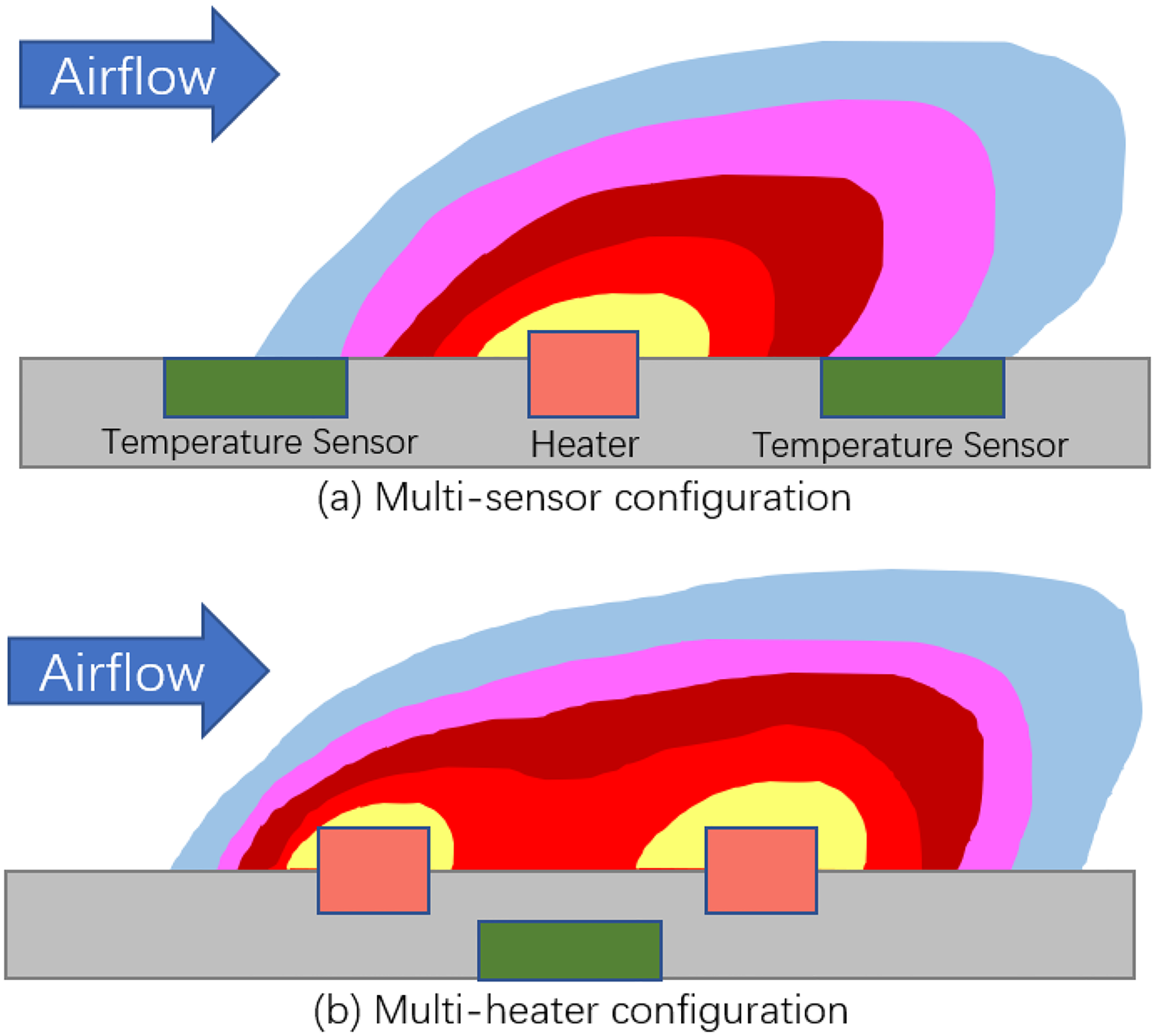
The bidirectional thermal anemometer is usually available in two configurations; the multi-sensor configuration estimates the flow rate by sensing the temperature difference at a given heating power, while the multi-heater configuration senses the flow rate by the difference in heating power at a constant relative ambient temperature.

Sliding window average denoising

Thermal anemometers measurement noise usually depends on the characteristics of the sensor itself and the complex turbulence around the sensor. Usually, the circuit noise and vibration has homoscedasticity characteristics (same or similar variances over the entire period) and the complex turbulence can also be regarded as having local homoscedasticity, (e.g. Figures 6 and 8). For such signals, sliding window average denoising method is the most easily used to filter out noise. Consequently, the noise-filtered sensor measurement model can be written

\hat{m} = f (v_{a})

(2)

Linear model

A commercially available anemometer usually has a reasonable measurement linearity, so we consider the approximation function as a biased linear function.

v_{a} = \frac{\hat{m} - b}{s} \in R

(3)

where

b

is the bias and

s

is the scale, which need to be identified from the filtered anemometer measurements

\hat{m}

and ground truth measurements of

v_{a}

. After combining many sampling data, we compose them in the form of a matrix:

[v_{a}] = A X (\hat{m}), A = (- b / s, 1 / s)

(4)

where

[v_{a}] = (v_{a} (t_{1}) \dots v_{a} (t_{N}))

and

X (\hat{m}) = (\begin{matrix} 1 & \dots & 1 \\ \hat{m} (t_{1}) & \dots & \hat{m} (t_{N}) \end{matrix})

contain ground truth air velocity measurements and anemometer measurements at different sampling times

t_{1}, \dots, t_{N}

, respectively. Ground truth air velocity measurements are provided by a SLAM system, as discussed later in Section Implementation & Results. Minimizing the squared sum of estimation errors

‖ [v_{a}] - A X (\hat{m})) ‖^{2}

(5)

gives the least squares estimator

\hat{A} = [v_{a}] X (\hat{m})^{T} (X (\hat{m}) X (\hat{m})^{T})^{- 1}

(6)

After identification of

A

, the air velocity estimate associated with a measurement

m

is thus given by:

{\hat{v}}_{a} = \hat{g} (m) = \hat{A} (1, m)^{T}

3D triaxial anemometer sensor

In this work, we built a triaxial sensor composed of three anemometers mounted in an orthogonal configuration, as shown on Figure 1. The objective is to estimate the 3D velocity/air-velocity. The following notation is used:

$I$ is an inertial frame.

$B$ is a body frame (i.e., attached to the MAV), with center at the MAV’s center of mass $G$ . The rotation matrix from $B$ to $I$ is denoted as $R$ and it satisfies the equation $\dot{R} = R [ω]_{\times}$ with $ω$ the angular velocity vector expressed in body frame and $[ω]_{\times}$ the skew-symmetric matrix associated with the cross product by $ω$ .

$S$ is a sensor frame (i.e., attached to the triaxial anemometer sensor), with center at the sensor’s center $C$ . The constant rotation matrix from $S$ to $B$ is denoted as $R_{0}$ and the vector of coordinates of $C$ in the body frame $B$ is denoted as $δ$ .

$V^{G}$ denotes the coordinates, in inertial frame, of the velocity vector of $G$ (i.e., the MAV’s velocity vector).

$V_{w}$ denotes the coordinates, in inertial frame, of the wind speed vector.

The objective is to estimate the MAV’s air-velocity vector

V_{a}^{G} = V^{G} - V_{w}

Let $V^{C}$ denote the coordinates, in inertial frame, of the velocity vector of $C$ . We have $V^{C} = V^{G} + R (ω \times δ)$ and thus

V_{a}^{C} : = V^{C} - V_{w} = V_{a}^{G} + R (ω \times δ)

where

V_{a}^{C}

denotes the air-velocity vector at the sensor center

C

, expressed in inertial frame. Using the linear model proposed in Section Linear model, the triaxial anemometer sensor provides the components of this vector in the sensor frame

S

. Since the rotation matrix from sensor frame to inertial frame is

\bar{R} = R R_{0}

, the vector of sensor measurements is

\begin{matrix} {\bar{V}}_{a}^{C} = {\bar{R}}^{T} V_{a}^{C} & = & {\bar{R}}^{T} V_{a}^{G} + {\bar{R}}^{T} R (ω \times δ) \\ = & R_{0}^{T} (R^{T} V_{a}^{G} + ω \times δ) \end{matrix}

which is equivalent to

R^{T} V_{a}^{G} = R_{0} {\bar{V}}_{a}^{C} - ω \times δ

(7)

In the following section we propose a deep learning-based solution to estimate

R^{T} V_{a}^{G}

from the vector of triaxial sensor measurements

{\bar{V}}_{a}^{C}

and the gyroscope measurement

ω

. The constant parameters

R_{0}

and

δ

in the above relation will be implicitly estimated by the neural network. For the MAV used in this work,

R_{0}

is probably close to the identity matrix but no calibration was performed.

Deep learning-based prediction with airflow

Model-based and data-driven solutions are two different state-estimation methods, each of which has different advantages. The model-based approach usually employs Kalman filters^12,15 to fuse multiple sensor data, low-pass filters¹¹ to reduce noise, or construct dynamical models² to extract airflow speed terms by referring to other measurements, respectively. A data regression method is employed by Müller et al.,¹⁰ and a deep learning-based method is employed by Tagliabue and How.¹⁹ Kalman-based filters are typically the most efficient and reliable for fusing multi-sensor data, while deep learning-based methods have better performance for extracting data features, denoising, and data regression. Turbulence causes heteroscedastic disturbance noise (e.g on Figure 6), which calls for data-driven approaches to identify temporary noise characteristics. In addition, the induced airflow on multi-rotor MAVs leads to regular coupling of measurement data from anemometers in different directions. Therefore, in this section we present our deep learning-based method, which is able to learn local noise features and thus perform denoising, compensate for unknown constant parameters ( $R_{0}$ and $δ$ ), and decouple the nonlinear relationship between data by deep learning a large amount of measurement data. We use a neural network composed of 1D convolution layers and Gated Recurrent Unit (GRU) layers.²⁰

Inputs & outputs

Due to the difficulty to obtain ground truth air velocity measurements, experiments are performed indoor, under the assumption of no ambient wind. Thus the MAV’s velocity is equal to its air velocity. According to the Equation (7), the inputs consist of a sequence of the anemometer airflow measurement data and a sequence of angular velocity measurements collected during a time window. Note that we have tried to add accelerometer measurements and motor commands as input of the neural network, but it has led to over-fitting. Inputs (resp. outputs) of the network are expressed in the sensor frame (resp. body frame) in order to keep the network invariant with respect to the vehicle’s orientation. This is important in order to reduce the complexity of the network and the amount of training data.

Neural network architecture

The architecture of the neural network is presented on Figure 5. The global architecture (Sub-Figure 5b) is composed of one scaling layer, two convolution layers, two GRU layers, and one fully connected layer (aka. output layer). The raw anemometer airflow measurement data and the raw gyroscope measurements are first processed by the scaling layer (Sub-Figure 5d). In this figure, the bias and the scale are those of the linear model presented in the previous section, and obtained by least-square minimization. Note that for the linear model identification, i.e., identification of scale and bias, anemometer measurements filtering has been performed, but of course the non-filtered raw data is used here as input of this scaling layer. Along the time series, the angular velocity data is stacked together with the transformed airflow data. Then, two layers of 1D convolution network (Sub-Figure 5a) are used for denoising, where the number of filters is equal to 16, the kernel size is equal to 5, the stride is equal to 1, the activation function is the rectified linear unit (ReLU),²¹ and the input and output sequences are of the same length by padding with zeros. The output of the second convolution layer serves as the GRU layer input. Then, two layers of GRU network (Sub-Figure 5c) with 16 units are stacked on top of convolution layers to extract deep features and to decouple the induced airflow from flight speed. Compared to Long-Short Term Memory (LSTM),²² GRU has fewer learnable parameters and thus less risk of over-fitting.²⁰ Eventually, an output layer with only three outputs is used to integrate the deeply processed information to produce the final flight speed prediction. The neural network is built upon TensorFlow.²³

Figure 5.

Neural network architecture.

Implementation & results

We present in this section implementation details and flight tests’ results of the proposed approach. To verify the robustness of the proposed approach with respect to the sensors architecture and training conditions, we performed two validations. The first validation was performed with the sensors configuration shown on Figure 1 (with three anemometers) and with flight trajectories generated in automatic flight mode (trajectory tracking) with ground-truth provided by a visual SLAM module. The second validation was performed with a slightly different sensors’ configuration (with four anemometers) and with flight trajectories generated in manual flight mode and ground-truth provided by a MoCap system. The trajectories obtained in the latter case where less repeatable and more aggressive than those obtained in the former. We detail in the following subsections the implementation details and results evaluation for the first set-up (automatic flight mode). In a last subsection, we provide additional information concerning the second set-up (manual flight mode).

Implementation details

We collect data on the custom-built MAV flight platform of Figure 1 with a frame of 15x20x20cm and weight about 500g. The MAV is equipped with Pixhawk 4 open source flight control board (STM32f7), D435i binocular depth camera, and Khadas Vim 3 SBC (6-core ARM 2.4GHz).

The open source flight control system PX4 runs on Pixhawk 4 and contains a 4-loops cascade PID controller, an Extended Kalman Filter (EKF) based state estimator, and uses the mavlink protocol to communicate with Vim 3 via the serial port. All components run in a ROS system on Vim 3 and communicate with an off-board laptop via wifi 5.

We use the thermal mass flow sensors SFM3000-200 from Sensirion AG. The sampling rate of 200Hz in the first evaluation (400Hz in the second) and the high speed I2C communication interface make it easy to acquire data. In this first evaluation, the flight data has been collected on different days in automatic flight mode in a standard gymnasium. A trajectory generator ROS node commands the vehicle to follow a reference trajectory that includes a circular spiral and a figure-of-8 spiral with a radius of 2 meters and an undulation height of 1 meter. The takeoff operation is also commanded by the ROS node during the automatic trajectory tracking. The ground truth velocity is provided by the EKF based on the ORB-SLAM3⁵ output and the IMU measurements. The EKF relies on the accelerometer measurement model.

The low priority of the data logging, due to the limitations of the autopilot hardware, would lose data randomly at different moments, but the total lost data would not exceed $2 %$ of the total. For this reason, we compensated for the missing ground truth data using a sliding window average cubic polynomial fitting method, while we approximated the missing raw sensor measurements using a linear interpolation method. We do not have statistics of slam accuracy, but the comparison⁴ shows that orb-slam3 exhibits performances similar to other state-of-the-art slam methods.

Neural network training

We divide the collected data into the training set (four flights data with a total of 20.18 minutes), validation set (two flights data with 14.47 minutes), and test set (one flight data with 4.04 minutes). To compensate for the differences in flying conditions on different days (air temperature, humidity, pressure, etc), both the training data-set and the validation data-set contain multiple flight data from different days. The batches of sequences are created by sliding a 2.5 seconds time window which contains 500 data. The batch size has been set as 512, and we use the Adam with Triangular Cyclic Learning Rate (CLR)²⁴ as the optimizer, which periodically increases and decreases the learning rate during the training. Early stopping is also used to avoid over-fitting.

Anemometer measurement noise characteristics

Figure 6 displays air-velocity estimates along the sensor front direction obtained with the linear model, before filtering (blue) and after filtering (red). The flight is composed of five different flight phases performed in automatic flight mode: takeoff, circular spiral trajectory, figure-of-eight spiral trajectory, vertical flight, and landing. The trajectory plots are shown on Figure 7, where the blue curve is the trajectory and the gray curves are its projection onto the $x$ , $y$ , and $z$ axes. We have used here a sliding window of length 19 to generate delay-free smooth data and obtain better noise characteristics. Of course, this sliding window is not used online for the air velocity estimation. The error statistics are presented on Figure 8, which shows that the anemometer measurements present a Gaussian white noise characteristic in the whole and Figure 6 shows that the measurements locally present a disturbance characteristic related to the flight state.

Figure 6.

Sliding window average denoise. [Top] The air-velocity estimate with the linear model in the Sensor Front direction before filtering (blue) and after filtering (red). [Bottom] The filtered noise shows that it presents almost homoscedasticity over the entire period, while locally, especially when the flight speed direction changes, it presents heteroscedasticity from the whole.

Figure 7.

Trajectories in NED frame during takeoff, circle spiral, figure-of-8 spiral, vertical flight, and landing in order from left to right.

Figure 8.

Histogram of the statistical distribution of the filtered noise. Generally, the noise presents Gaussian white noise characteristics with the mean of $2.5 \times 10^{- 3} m / s$ and the std of $0.04 m / s$ .

Prediction of linear model and GRU model

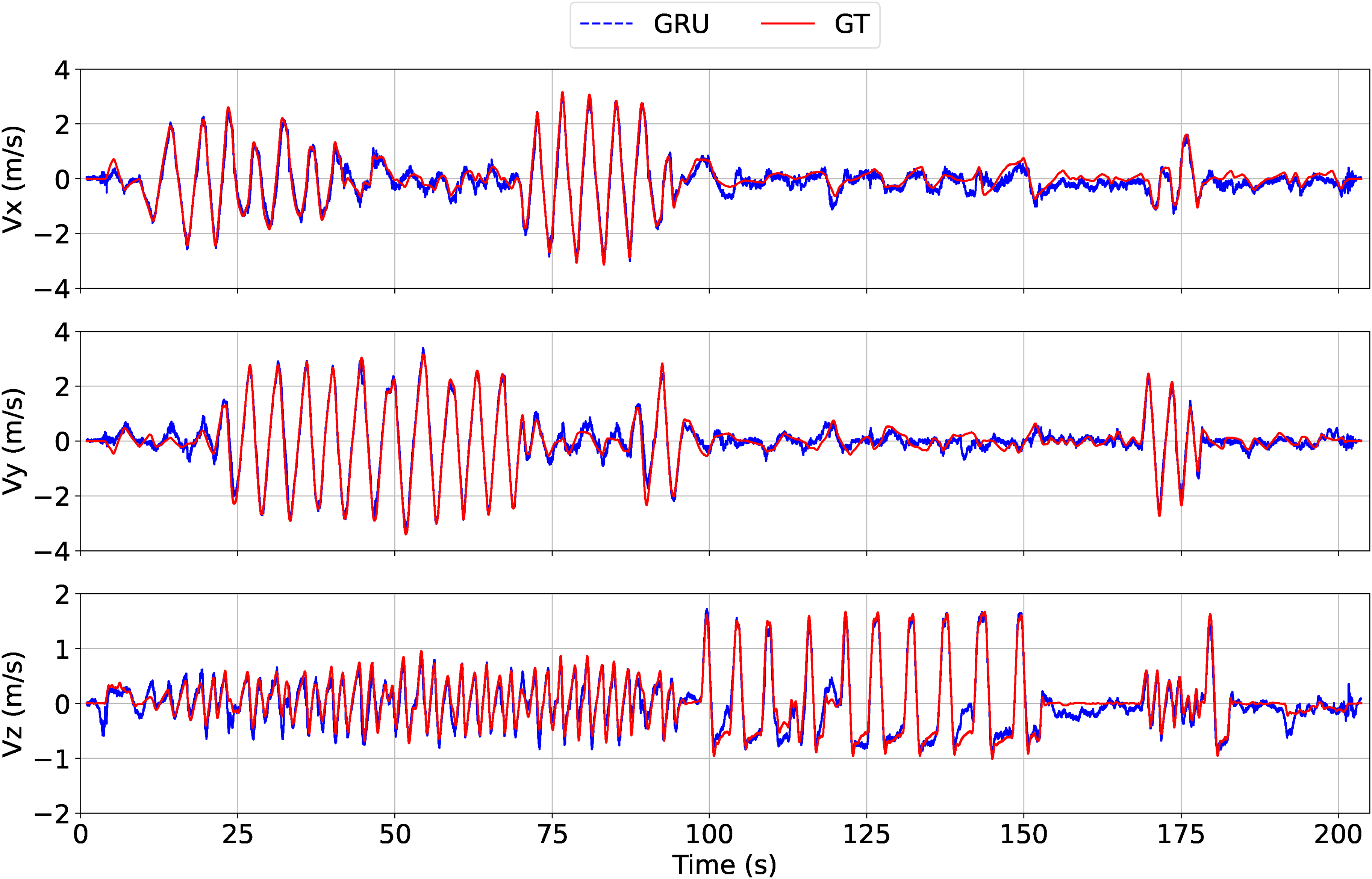
For the test flight, the trajectory of Figure 7 was used. The prediction results are shown on Figure 9, where we compare the flight speed prediction of the linear model of Section Linear model (green dashed line) with the flight speed prediction of the GRU model (blue dashed line) and the ground truth flight speed (red solid line). Along the time axis, in order, the five flight phases are takeoff, circular spiral, figure-of-8 spiral, vertical flight, and landing, each marked with a different color.

Figure 9.

Five flight phases are respectively in chronological order the take-off (<30s), the circular spiral trajectory (40s–110s), figure-of-eight trajectory (120s–170s), vertical flight (180s–230s), and the landing (240s–250s). The flight speed prediction of the identified linear model without removing the noise (green) vs. that of the learning-based model (blue) vs. the ground truth flight speed from V-SLAM (red). All is expressed in Body-FRD frame.

The parameters of the identified linear model are presented in Table 1, where Sensor-F, Sensor-R, and Sensor-D stand for the Front, Right, Down directions in the sensor frame respectively. As expected from the symmetry of the system, parameters for the Sensor-F and Sensor-R are very close. Concerning the vertical direction (i.e., Sensor-D), we identified this model using only flight data from hovering and vertical flights, so as to avoid the impact of horizontal flight velocity on the induced velocity. When the horizontal flight is dominant, the linear model estimation in the F-R direction shows essentially the consistency with the ground truth, while the resulting induced flow causes bias in the D-direction estimation. When vertical flight is dominant, the strong variations of the induced speed are measured by the anemometer sensor ahead of the ground truth speed estimation based on the visual SLAM, thus leading to the linear model estimation in D-direction being ahead of the ground truth flight speed estimation. The vertical flight speed also shows a slight coupling characteristic with the horizontal measurements.

Table 1.

Parameters identification with linear regression.

Parameters	Sensor-F	Sensor-R	Sensor-D
Bias b	−0.0020	0.0154	−0.2143
Scale s	0.3100	0.2984	0.1420

Figure 10 shows the flight speed prediction error of the linear model w.r.t the ground truth versus the flight speed prediction error of the GRU model w.r.t the ground truth in each direction. The variances of the GRU model in each direction are 0.0111, 0.0132, 0.0143, respectively, while that of the linear model in the F-R direction are 0.0421 and 0.0377 respectively.

Figure 10.

The flight speed prediction error of linear model w.r.t the ground truth (green) vs. the flight speed prediction error of deep learning-based model w.r.t the ground truth (blue). The variances of thei GRU model in the each direction are 0.0134, 0.0133, 0.0139, while the variances of the linear model in the F-R direction are 0.0421, 0.0377, respectively.

We summarize the results as follows: (1) The prediction results of GRU largely overlap with the ground truth, better than linear model, which indicates that the neural network successfully discovers patterns in the data. (2) The GRU model flight speed prediction curve is smooth, which indicates that the neural network identifies the noisy feature and thus performs denoising process. (3) The anemometer measurements in the D-direction implicitly contain the induced flow speed, which is coupled with the flight state, and which is usually difficult to predict and the linear model performs poorly for the prediction of the flight speed in trajectory tracking. The GRU model shows better performance, however, especially during the takeoff and landing phases. This is testimony to the GRU model’s robustness. (4) For the flight speed prediction in the F-R direction, both the linear model and the GRU model match the ground truth well but Figure 10 shows that the GRU model largely outperforms the linear model.

Integral drift of GRU model flight speed prediction

To evaluate the possibility to use the obtained velocity estimates for odometry (i.e., displacement estimation), we performed integration of the velocity estimates. Since these estimates are given in body frames, they were first transformed in inertial frame using the rotation matrix provided by the EKF, and then numerically integrated. Figure 11 displays the drift of the so-obtained odometry estimation with respect to the SLAM-based ground truth. Figure 12 shows the trajectory obtained by odometry versus the ground truth trajectory given by the SLAM, during different flight phases, where the red curves are the same as those shown in Figure 7. We summarize the results as follows: (1) The odometry drift, in term of Euclidean distance to the ground truth, based on integration of the flight speed estimates is about 3 cm per second on average. (2) We collected flight data on different days and the sensor setup composed of the three anemometers was unmounted at the end of each flying day. Therefore, there can be small differences between the data sets for the constant parameters $R_{0}$ and $δ$ . Such differences can bias a little bit the flight speed estimation. It is particularly demonstrated in the z-axis direction during the hovering in Figure 11.

Figure 11.

The integral drift of flight speed prediction by using GRU model in Body frame during 5 flight phases.

Figure 12.

The trajectory of the flight speed integral predicted by the GRU model versus the real trajectory in ENU frame during takeoff, circle spiral, figure-of-8, vertical flight, and landing in order from left to right.

GRU model prediction in manual flight mode

During teleoperation, MAVs are operated manually and this may lead to aggressive maneuvers. Previously, we used visual SLAM to provide localization services and thus collected multiple flight data sets in automatic flight mode. In order to verify that the GRU-based neural network model is robust and can cope with more aggressive and irregular flight trajectories, we performed manual flights. Beside this difference, we used a MoCap positioning system to provide localization services for the ground truth, instead of the SLAM-based ground truth used in the previous validation. Finally, we also used another sensor hardware architecture, with four anemometers instead of three, where two of them are aligned with the (body-fixed) vertical direction, as shown on Figure 13 below. Except for these differences, the procedure for training and evaluation is the same as in the previous validation with SLAM-based ground truth. Part of the flight data is used to train the GRU-based neural network with the same architecture as used before. The flight speed prediction results on the test set are shown in Figure 14 and the prediction error is shown in Figure 15. Note that the flight speeds are significantly higher than those of the first validation and exhibit significant velocity dynamics (i.e., accelerations). The results are consistent with those obtained in the first validation, and demonstrate the robustness of the GRU neural network-based model and its capacity to predict the flight speed in this more challenging scenario.

Figure 13.

Sensors’ layout for the second validation, with two anemometers in the (body-fixed) vertical direction.

Figure 14.

GRU model flight speed prediction (blue) versus the ground truth flight speed (red) in Body frame with manual flight (i.e., second validation).

Figure 15.

The flight speed prediction error of GRU model w.r.t the ground truth.

Conclusion & future work

In this work we addressed the velocity/air velocity estimation problem aboard MAVs based on thermal anemometer measurements. The proposed solution uses a set of sensors mounted in a triaxial orthogonal configuration and combines a simple analytical model with a neural network. By performing all computations in body and sensor frames, the problem is invariant with respect to rotations, which reduces the complexity of the neural network and the amount of required training data. Validations show that the neural network brings significant benefits in term of denoising and compensation of induced-flow.

Perspectives include using other sensors available on-board MAVs, such as accelerometers and barometers, to further improve speed prediction, or exploiting anemometer measurements for obstacles detection. Wind field estimation and aerodynamic model identification are additional perspectives of this work.

Footnotes

Acknowledgements

This work was supported by the French ANR Project DACAR.

The first author is funded by the China Scholarship Council (CSC) from the Ministry of Education of P.R. China.

The authors want to thank Dr. Jorge ARIZAGA and Dr. Pedro CASTILLO from Heudiasyc at UTC, Compiègne, France, for giving them access to the Heudiasyc flying arena and providing support for the manual flight tests exploited in this paper.

The authors want to thank Prometheus^a platform support.

Declaration of conflicting interests

The author(s) declared no potential conflicts of interest with respect to the research, authorship, and/or publication of this article.

Funding

The author(s) disclosed receipt of the following financial support for the research, authorship, and/or publication of this article: The authors received financial support from the French ANR Project DACAR for the research in this article.

ORCID iDs

Ze Wang

Jingang Qu

Notes

References

Mohamed

Schwarz

. Adaptive kalman filtering for INS/GPS. J Geod 1999; 73: 193–203.

Sikkel

LNC

de Croon

De Wagter

, et al. A novel online model-based wind estimation approach for quadrotor micro air vehicles using low cost MEMS IMUs. In: 2016 IEEE/RSJ International Conference on Intelligent Robots and Systems (IROS), 2016, October, pp. 2141–2146. IEEE.

Zhang

Singh

. LOAM: Lidar odometry and mapping in real-time. In: Robotics: Science and Systems 2014, July; (Vol. 2, No. 9, pp. 1-9).

Sharafutdinov

Griguletskii

Kopanev

, et al. Comparison of modern open-source visual SLAM approaches. arXiv preprint arXiv:2108.01654, 2021.

Mur-Artal

Montiel

JMM

Tardos

. ORB-SLAM: a versatile and accurate monocular SLAM system. IEEE Trans Robot 2015; 31: 1147–1163.

Letalenet

Morin

. Identification and evaluation of a force model for multirotor UAVs. In: 2020 IEEE International Conference on Robotics and Automation (ICRA), 2020, May, pp. 4280–4286, IEEE.

Brossard

Bonnabel

Barrau

. Denoising imu gyroscopes with deep learning for open-loop attitude estimation. IEEE Robotics and Automation Letters 2020; 5: 4796–4803.i.

Wang

Morin

. Deep learning flight speed estimation using thermal anemometers. In: 2022 International Micro Air Vehicle Conference (IMAV).

Bruschi

Piotto

Dell’Agnello

, et al. Wind speed and direction detection by means of solid-state anemometers embedded on small quadcopters. Procedia Eng 2016; 168: 802–805.

10.

Müller

Paul

Burgard

. Probabilistic velocity estimation for autonomous miniature airships using thermal air flow sensors. In: 2012 IEEE International Conference on Robotics and Automation, 2012, May, pp. 39–44, IEEE.

11.

Zahran

Zhuang

, et al. IMU/magnetometer/barometer/mass-flow sensor integrated indoor quadrotor UAV localization with robust velocity updates. Remote Sens (Basel) 2019; 11: 838.

12.

Hollenbeck

Nunez

Christensen

, et al. Wind measurement and estimation with small unmanned aerial systems (suas) using on-board mini ultrasonic anemometers. In 2018 International Conference on Unmanned Aircraft Systems (ICUAS), 2018, June, pp. 285–292. IEEE.

13.

Prudden

Fisher

Marino

, et al. Measuring wind with small unmanned aircraft systems. J Wind Eng Ind Aerodyn 2018; 176: 197–210.

14.

Tagliabue

Paris

Kim

, et al. Touch the wind: Simultaneous airflow, drag and interaction sensing on a multirotor. In: 2020 IEEE/RSJ International Conference on Intelligent Robots and Systems (IROS), 2020, October, pp. 1645–1652, IEEE.

15.

Zahran

Moussa

Sesay

, et al. A new velocity meter based on hall effect sensors for UAV indoor navigation. IEEE Sens J 2018; 19: 3067–3076.

16.

Deer

Pounds

. Lightweight whiskers for contact, pre-contact, and fluid velocity sensing. IEEE Robotics and Automation Letters 2019; 4: 1978–1984.

17.

Sazhin

. Novel mass air flow meter for automobile industry based on thermal flow microsensor. I. Analytical model and microsensor. Flow Meas Instrum 2013; 30: 60–65.

18.

Sparks

. MEMS pressure and flow sensors for automotive engine management and aerospace applications. MEMS for Automotive and Aerospace Applications 2013: 78–105.

19.

Tagliabue

How

. Airflow-Inertial Odometry for Resilient State Estimation on Multirotors. In: 2021 IEEE International Conference on Robotics and Automation (ICRA), 2021, May, pp. 5736–5743. IEEE.

20.

Cho

Van Merriënboer

Gulcehre

, et al. Learning phrase representations using RNN encoder-decoder for statistical machine translation. arXiv preprint arXiv:1406.1078, 2014.

21.

Nair

Hinton

. Rectified linear units improve restricted boltzmann machines. In: Icml, 2010, January.

22.

Hochreiter

Schmidhuber

. Long short-term memory. Neural Comput 1997; 9: 1735–1780.

23.

Abadi

Barham

Chen

, et al. TensorFlow: a system for Large-Scale machine learning. In: 12th USENIX symposium on operating systems design and implementation (OSDI 16), 2016, pp. 265–283.

24.

Smith

. Cyclical learning rates for training neural networks. In: 2017 IEEE winter conference on applications of computer vision (WACV), 2017, March, pp. 464–472. IEEE.

Airflow-based odometry for MAVs using thermal anemometers

Abstract

Keywords

SOURCE CODE

Introduction

Airflow sensors for MAVs

Thermal anemometer measurement model

Sliding window average denoising

Linear model

3D triaxial anemometer sensor

Deep learning-based prediction with airflow

Inputs & outputs

Neural network architecture

Implementation & results

Implementation details

Neural network training

Anemometer measurement noise characteristics

Prediction of linear model and GRU model

Integral drift of GRU model flight speed prediction

GRU model prediction in manual flight mode

Conclusion & future work

Footnotes

Acknowledgements

Declaration of conflicting interests

Funding

ORCID iDs

Notes

References