Sage Journals: Discover world-class research

Abstract

In the field of machine vision, the multi-solution problem of the perspective-three-point (P3P) camera pose estimation problem has been widely researched. Many researchers have tried to find unique solutions that will enable the use of the P3P method in practical applications such as the calibration of external parameters of a camera. Gao found a special case that is very simple and intuitive, but can only be used for a camera with a very large field of view. Therefore, it did not attract much attention. The purpose of this study was to analyse Gao's special case and use it for calibrating the external parameters of an omnidirectional camera, which is used widely because of its very large field of view. We first verify Gao's special case and extend its application. We then propose an iterative method for finding the unique solution. After this, we perform a simulation experiment to determine the effect of the configuration of the three control points on the accuracy of the unique solution. Finally, we use an application to examine the efficiency of the method.

Keywords

perspective-three-point problem multi-solution phenomenon unique positive solution external parameter calibration omnidirectional camera

1. Introduction

Determining the pose of a camera given the images of three known points in a 3D space is the classical perspective-three-point (P3P) problem [1], which is a sub-problem of the perspective-n-point problem. It has gained the most attention because it requires the least number of points of correspondence. It is widely used in some hypothesis-and-test architectures such as RANSAC [2], where it enhances the efficiency by reducing the number of hypotheses. It can also be used to obtain the original value for pose estimation using nonlinear refining methods. However, a drawback of the P3P method is the well-known multi-solution problem [1]. There are at most four possible positive solutions to the P3P problem. The multi-solution problem observably affects efficiency because it doubles the time required to tackle all the possible solutions equally [2].

The research on the multi-solution problem involves two cases of the P3P problem. First, the traditional case involves the use of three control points and three image points to determine the pose of a camera. In this case, we need to classify the number of solutions and determine the appropriate solution. In the second case, three control points are configurable in an application such as the calibration of the external parameters of a camera. In this case, we need to determine how to configure the control points to obtain a unique solution.

Research on the number of solutions and the solving method was started by Wolfe. Wolfe et al. [3] gave a geometric explanation of the camera-triangle configurations that produce one, two, three or four solutions by adopting the “canonical view.” Su et al. [4] proposed an algebraic analysis of the necessary and sufficient condition for a positive root number of the P3P problem.

In relation to research on unique solutions, Gao [5] proved that under the reality condition, if the angles between any two of the back-projection rays corresponding to the three control points are obtuse, the P3P problem can have only one solution. Because this special case requires the camera to have a very large field of view, it has not gained much attention. Zhou and Zhu [6] found that when the three control points form an isosceles triangle and the camera is within two special regions, the P3P problem will have a unique solution. Wang et al. [7] and Tang and Liu [8] extended the work of Zhou and Zhu [6]. They divided the 3D space by projecting the perspective centre on the plane that contained the control points and found seven unique solution regions. There were two basic assumptions in all these works[6 –8]: (1) the three control points form an isosceles triangle, and (2) the approximate relative poses between the control points and camera are known.

In recent years, many types of omnidirectional cameras with large field of view (FOV) vision systems have become widely used, which was one of the motivations for this study. We found that although Gao's special case is not useful for the conventional camera, it is suitable for an omnidirectional camera. In this study, we analyse and expand Gao's special case, and then propose an iterative method for obtaining a solution. We use simulation data to analyse the effect of the configuration of the three points on the solution accuracy. Further, we use a calibration application to examine the efficiency of the method.

2. Definition and notation

Many definitions have been proposed for the P3P problem. Here, we use the simple version[4] shown in Fig.1. Given three rays, r_a,r_b, and r_c, starting from the centre of perspective (CP) point O, try to find three points, A,B, and C on the rays such that they satisfy the condition dist(A,B)=L_ab, dist(A,C) = L_ac, and dist(B,C) = L_bc,

Figure 1.

Simple model of P3P problem.

where L_ab, L_ac, and L_bc denote the original distances between the three control points and dist(A,B) denotes the Euclidean distance between points A and B. These three points are parameterized with their distances to the CP, denoted as t_a,t_b and t_c, which are the only unknown variables that need to be solved. The angle between two rays is denoted as θ_ab for example.

Based on this notation Gao's Theorem 9 in paper [5] can be expressed as follows:

Under the reality conditions, if θ_ab, θ_ac, and θ_bc are obtuse, then the P3P problem can only have one solution. Furthermore if < ACB < θ_ab, <ABC < θ_ac, <BAC < θ_b,c, then the P3P problem has a unique solution.

There are two results in Gao's Theorem, the first one shows that when the three angles(θ_ab, θ_ac, and θ_bc) are obtuse, the P3P problem can at most have one solution. The second result is a sufficient condition for the P3P problem having a unique solution.

3. Special cases of a unique positive solution

Gao [5] found the special unique solution case using a geometrical method. However, in this section, we propose a new definition for the special case and prove it using basic algebra.

3.1 A. Special case of the P3P problem

Definition: If the angles between any two of the back-projection rays (r_a,r_b, and r_c) corresponding to the three control points are obtuse, the problem is a special case and is called an obtuse P3P problem.

Result 1: If an obtuse P3P problem has a positive solution, then it has a unique solution.

Proof:

Applying the cosine theorem to triangles ΔAOB, ΔAOC, and ΔBOC gives us

L_{a b}^{2} = t_{a}^{2} + t b^{2} - 2 t_{a} t_{b} cos θ_{a b}

(1)

L_{a c}^{2} = t_{a}^{2} + t_{c}^{2} - 2 t_{a} t_{c} cos θ_{a c}

(2)

L_{b c}^{2} = t_{b}^{2} + t_{c}^{2} - 2 t_{b} t_{c} cos θ_{b c}

(3)

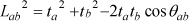
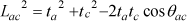
Using these three equations, we eliminate t_b and t_c.

Derived from (1)

{(t_{b} - t_{a} \cos θ_{a b})}^{2} = L_{a b}^{2} - t_{a}^{2} \sin^{2} θ_{a b}

Because t_b > 0 and θ_ab > 90° we have

t_{b} = t_{a} \cos θ_{a b} + \sqrt{L_{a b}^{2} - t_{a}^{2} \sin^{2} θ_{a b}}

(4)

Similarly, from (2)

t_{c} = t_{a} \cos θ_{a c} + \sqrt{L_{a c}^{2} - t_{a}^{2} \sin^{2} θ_{a c}}

(5)

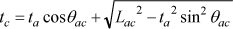
Substitute (4) and (5) into (3), and let

f (t_{a}) = t_{b}^{2} + t_{c}^{2} - 2 t_{b} t_{c} \cos θ_{bc} - L_{bc}^{2}

(6)

Now, the P3P problem translates to solving the equation f(t_a) = 0.

We now compute the derivative of f(t_a)

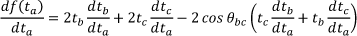
\frac{d f (t_{a})}{d t_{a}} = 2 t_{b} \frac{d t_{b}}{d t_{a}} + 2 t_{c} \frac{d t_{c}}{d t_{a}} - 2 \cos θ_{b c} (t_{c} \frac{d t_{b}}{d t_{a}} + t_{b} \frac{d t_{c}}{d t_{a}})

(7)

Then, the derivative dt_b/dt_a and dt_c/dt_a can be computed from (4) and (5),

\frac{d t_{b}}{d t_{a}} = \cos θ_{a b} - t_{a} \sin^{2} θ_{a b} / \sqrt{L_{a b}^{2} - t_{a}^{2} \sin^{2} θ_{a b}} < 0

(8)

\frac{d t_{c}}{d t_{a}} = \cos θ_{a c} - t_{a} \sin^{2} θ_{a c} / \sqrt{L_{a c}^{2} - t_{a}^{2} \sin^{2} θ_{a c}} < 0

(9)

Substitute (8) and (9) into (7), we then have df(t_a)/dt_a < 0, which means there is a monotone decreasing relationship between f(t_a) and t_a when t_a > 0. Thus, if the obtuse P3P problem has a positive solution, which also means equation f(t_a) = 0 has a positive solution, then it has a unique solution.

Result 2: An obtuse P3P problem has a unique positive solution if and only if

∠ ACB \leq θ_{a b}, ∠ ABC \leq θ_{a c}, ∠ BAC \leq θ_{b c}

Proof:

As can be seen from Fig.1, to have physical meaning, solution t_a should be between t_{a min}=0 and t_{a max} =Min(L_ab, L_ac). From the proof of Result 1, we know that t_a and f(t_a) have a monotone relationship, so

When t_a=t_amin = 0, according to (4)and(5), t_b = L_ab,t_c=L_ac. Then We have

\begin{array}{l} f {(t_{a})}_{m a x} = f (t_{a m i n}) \\ = L_{a b}^{2} + L_{a c}^{2} - L_{b c}^{2} - 2 L_{a b} L_{a c} c o s θ_{b c} \\ = 2 L_{a b} L_{a c} cos (∠ BAC) - 2 L_{a b} L_{a c} c o s θ_{b c} \end{array}

(10)

If we assume L_ab < L_ac, so t_amax = L_ab.

When t_a = t_amax = L_ab, according to (4) and $θ_{ab} > \frac{π}{2}$

\begin{array}{l} t_{b} = L_{a b} \cos θ_{a b} + \sqrt{L_{a b}^{2} - L_{a b}^{2} \sin^{2} θ_{a b}} \\ = L_{a b} \cos θ_{a b} - L_{a b} \cos θ_{a b} = 0 \end{array}

Substitutet_b = 0 in (3) and t_c > 0, we have t_c = L_bc

So we have

f {(t_{a})}_{m i n} = f (t_{a m a x}) = 0

(11)

Because the monotoneproperty if and only if f(t_a)_min <= 0 <= f(t_a)_max, the obtuse P3P problem will have a positive solution, and the solution will be a unique positive solution according to Result 1.

So according to (10),(11) $0 < ∠ B A C < π, \frac{π}{2} < θ_{b c} < π$ we have

\begin{array}{l} f {(t_{a})}_{m i n} \leq 0 \leq f {(t_{a})}_{m a x} \\ \Leftrightarrow 0 \leq 0 \leq 2 L_{a b} L_{a c} \cos (∠ BAC) - 2 L_{a b} L_{a c} c o s θ_{b c} \\ \Leftrightarrow \cos (∠ BAC) \geq c o s θ_{b c} \\ \Leftrightarrow ∠ B A C \leq θ_{b c} \end{array}

Similarly, we can prove <ACB ≤ θ_ab and ∠ABC ≤ θ_ac.

3.2 Solving the unique solution

From the previous proof, we know that solving equation f(t_a) = 0 is the key. The monotone property of f(t_a) simplifies the solution to a great extent. We choose an iterative root-finding method called the false position method or regulafalsi method, which combines features from the bisection method and secant method[9]. The basic idea of this method is to start with two points, a₀ and b₀, such that f(a₀) and f(b₀) have opposite signs, which implies by the intermediate value theorem that function f has a root in the interval [a₀,b₀], assuming continuity of function f. The method proceeds by generating a sequence of shrinking intervals [a_k,b_k] that contain a root of f. In our case, we choose a₀ = t_amin=0 and b₀ = t_amax =Min(L_ab,L_ac). The pseudo-code is as follows[10]:

{ a = 0; b=Min(L_ab,L_ac);

c = \frac{a f (b) - b f (a)}{f (b) - f (a)};

; k = 0; m = 5; While(k<m) { If(Sign(f(b)) == Sign(f(c))) b = c; Else a = c;

c = \frac{a f (b) - b f (a)}{f (b) - f (a)};

; k = k + 1; } }

3.3 Discussion

In general, the two criteria used to determine whether a P3P problem has a special unique solution case are as follows: (1) whether it is an obtuse P3P problem and (2) whether it satisfies the conditions of result 2. However, for some applications with known data correspondence, the first part is sufficient using result 1. However, these two criteria are easy to define, for example, whether the problem is obtuse can be determined from the sign of the dot product of two rays. Moreover, it should be noted that thanks to the large FOV of an omnidirectional camera, it will be easy to satisfy these criteria, as discussed in the following section.

4. Experimental results

In the last section, we proposed a method to determine a unique solution. In this section, we describe an experiment used to determine how the configuration of the three control points affects the accuracy of the unique positive solution. A catadioptric camera is used, whose system structure is shown in Fig.2. We set a world frame with the checkerboard pattern and a camera frame at the base of the mirror. The relative pose (represented by rotation angles in rad and translation components in mm as(θ_x,θ_y,θ_z,T_x,T_y,T_z,)) of the camera frame to the world frame is computed and compared with the ground truth.

Figure 2.

Model of non-central catadioptric camera.

In the simulation, the configuration of the three control points is set as shown in Fig.3, where O_i, i= 1,2,3 represent the three control points on the checkerboard pattern, O' is the projection of CP, d is the distance between O' and O_i, h is the height of the camera above the checkerboard pattern, and θ is the angle between 0'Q₂ and 0'Q₃. Fig.4 shows the simulation images used in the experiments.

Figure 3.

Configuration of camera and three points.

Figure 4.

Computer simulated images used in experiments.

4.1 Performance in relation to noise level

In this experiment, the three control points are chosen in the world coordinate system with d = 4m, h = 1m, and θ = 2π/3 (red points in the first part of Fig.4), and the ground truth of the relative pose is (0.1489,-0.1953,0.5,265,264,1023). Gaussian noise with a zero mean and varied standard deviation is added to the three corresponding image points. We vary the noise level of the three image points from 0.1 to 4 pixels. For every noise level, we perform 200 independent trials. The estimated pose parameters are then compared with the ground truth and the results shown are the average absolute errors. Figure 5 shows that the errors increase almost linearly with increasing noise level, and the local small volatility of the curves is mainly caused by the nonlinear properties of the P3P problem and the randomness of the experiment. For σ = 0.5 (which is the normal noise in a practical application), the error is (0.0026,0.0024,0.0017,16.937,18.5373,11.7186).

Figure 5.

Error vs. noise level of image points.

4.2 Performance in relation to distances of three points

In this experiment, we verify the accuracy of the unique positive solution with respect to d. The ground truth of the pose of the camera is (0,0,0,0,0,1024), h = 1m, and θ = √2π/3. Using simple geometry, we find that we should let d > √2h to meet the obtuse constraint of θ_ij. We then vary d from 2m to 9m and also add a Gaussian noise with 0 mean and 0.5 pixel standard deviation to the three image points (red points second part of Fig.4). Similar to experiment 1, we perform 200 independent trials for every d and measure the absolute error for every parameter of the pose. Fig.6 shows that the errors of the rotation angles decrease linearly with d, while the errors of the translation components increase linearly with d. This phenomenon is as expected. According to [11], faraway calibration points are good for determining the direction, whereas nearby points are suitable for determining the position. Therefore, the average back-projection error of 441 corner points on the checkerboard pattern (blue points in second part of Fig.4) is computed to test the integrated effect of d. Fig.7 shows that the back-projection error decreases with d, which indicates that the faraway points are better than the nearby points.

Figure 6.

Error vs. distance to centre.

Figure 7.

Back-projection error vs. distance to centre.

4.3 Performance in relation to angles of three rays

In this experiment, we examine the effect of θ on the accuracy of the unique positive solution. To satisfy the obtuse constrains, the value of θ should be within the range of $[\begin{matrix} 2 \arcsin (\frac{\sqrt{2 (h^{2} + d^{2})}}{2 d}), & 2 π - 4 \arcsin (\frac{\sqrt{2 (h^{2} + d^{2})}}{2 d}) \end{matrix}]$ . We set d = 2m,h=1m, and varied θ from 1.902 to 2.402 (red points in the third part of Fig.4). The result also shows the average absolute error of closure of 200 independent trials for every θ. In the results shown in Fig.8, we can see that the different values of θ do not affect the accuracy, which means we can ignore the angle when configuring the three control points.

Figure 8.

Error vs. angles of three rays.

5. Application

The method of this unique solution of P3P problem can be used in two types of application. The primaryone is the calibration of the omnidirectional camera. The second potential application is the robot localization application which is based on the feature map and RANSAC [2] method using an omnidirectional camera. In fact, the P3P method is widely used by the RANSAC method, because it needs the least number of samples, and our unique solution P3P method can reduce the sample number further.

However, because in the calibration application we can assign the configuration of the three calibration points, which is the main concern of this paper, so a calibration of the omnidirectional camera of soccer robot is discussed as follows.

5.1 Calibration of omnidirectional camera for a soccer robot

The left part of Fig.9 shows a scene of the soccer robot competition and the right is the omnidirectional image capture by the omnidirectional camera system. Using this omnidirectional image, the soccer robot obtains all the needed information to determinate what to do. One of the most important things is the real distance between the robot and other object on the field, such as the ball, other robots, the goal and so on. So distance mapping from the image distance to the real distance has to be calibrated. Usually, this calibration can be divided into two parts, the internal parameters' calibration and external parameters' calibration. The internal parameters include the camera parameters and the relative pose between camera and mirror, whose calibration can be referred to in[12]. The external parameters are the relative pose between the mirror andthe field, which can be calibrated using the P3P methodproposed in this paper.

Figure 9.

A scene of soccer robot competition and a sample of the omnidirectional image.

Computer synthetic data was used, because the ground truth was easy to obtain in a simulation environment and the internal parameters are assumed to be known.

To make the calibration more practicable, we use a feature point on the field, such as the cross point of the lines, to be the calibration point. According to 4.2,enlarging the distance between the three calibration points can decrease the back-projection error, we choose the three points as the red point on the left part of Fig.10, and put the robot in the yellow point position. Notice that, according to the 4.3, the value of three angles has little influence on the precision, so the robot need not be exactly at the centre of the three points.

Figure 10.

The calibration points and the synthetic omnidirectional image.

The calibration flow is as follows:

Step 1. According to the image coordinates of those three calibration points and using the internal parameters we compute the three ray (r_a, r_b, r_c) in the mirror coordinate system.

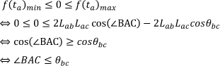
Step 2. Compute the angles (θ_ab,θ_ac, and θ_bc) and (<ACB, <ABC, <BAC), and then check the unique solution condition using Result 2. For example

θ_{a b} = \cos^{- 1} (r_{a}^{T} * r_{b}) .

Step 3. Compute the external parameters using the iterative method in 3.2

The calibration results are as follows:

The three rays are,

\begin{matrix} r_{a} = (- 0.98388, 0.003501, - 0.17882) \\ r_{b} = (0.609586, - 0.78562, - 0.10589) \\ r_{c} = (0.606732, 0.788428, - 0.10128) \end{matrix}

The angles are,

\begin{matrix} θ_{a b} = {125.7022}^{°}, θ_{a c} = {125.1751}^{°}, a n d θ_{b c} = {103.8170}^{°} \\ ∠ ACB = {56.3099}^{°}, ∠ ABC = {56.3099}^{°}, ∠ BAC = {67.3801}^{°} \end{matrix}

So the distribution of the three calibration points meets the unique solution conditions as Result2.

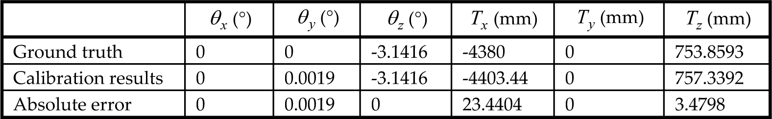
Finally, the computed external parameters are shown in Table 1. We can see that the errors of translation components are relatively bigger than the errors of the rotation components, which is the same as the result in Section 4.2 To show the precision of back-projection, we add some virtual cross lines on the soccer field, and generate an image as in Fig.11. Then we unwarp the omnidirectional image using the calibrated parameters. In Fig.12, the left part shows the unwrapped result and the right part has the true lines drawn on it. The unwrapped result shows the high precision of the back-projection.

Table 1.

Calibration result for external parameters.

	θ_y(°)	θ_z(°)	T_x (mm)	T_z (mm)
Ground truth	0	−3.1416	−4380	753.8593
Calibration results	0.0019	−3.1416	−4403.44	757.3392
Absolute error	0.0019	0	23.4404	3.4798

Figure 11.

The soccer field with some cross lines and the synthetic omnidirectional image.

Figure 12.

The unwrapped result and the unwrapped result with the true lines drawn on.

6. Conclusion

In this study, we proved and expanded Gao's special unique solution case for the P3P problem. This special case applies constraints directly on the angles between the three rays. Thus, it is very simple and intuitive, and is especially suitable for use with an omnidirectional camera. The iterative solving method used here is also simple and efficient, requiring less than 20 lines of Matlab code and less than five iterations to converge. Experimental results show that larger the distance of the three points, the better is the solution accuracy, however, the angles do not have a very large effect on the solution accuracy.

References

Haralick

R. M.

Lee

Ottenberg

(1994) Review and Analysis of Solutions of the Three Point Perspective Pose Estimation Problem. International Journal of Computer Vision.13 (3): 331–356.

Fischler

M. A.

Bolles

R. C.

(1987) Random sample consensus: A paradigm for model fitting with applications to image analysis and automated cartography. Communications of the ACM. 24 (6): 381–395.

Wolfe

W. J.

Mathis

Sklair

C. W.

(1991) The Perspective View of Three Points. IEEE Trans. Pattern Anal. Mach. Intell.13 (1): 66–73.

(1998) Necessary and Sufficient Condition of Positive Root Number Of Perspective-Three-Point Problem. Chinese Journal of Computer. 21 (12): 1084–1090.

Gao

Hou

Tang

(2003) Complete Solution Classification for the Perspective-Three-Point Problem. IEEE Trans. Pattern Anal. Mach. Intell. 25 (8): 930–943.

Zhou

Zhu

(2003) A note on unique solution conditions of the P3P problem. Chinese Journal of Computer. 26 (12): 1696–1701.

Wang

Yao

(2006) Some Discussion on the Conditions of the Unique Solution of P3P Problem. In Proceedings of the 2006 IEEE International Conference on Mechatronics and Automation. Luoyang, Henan 25–28, June 2006; 205–210

Tang

Liu

(2009) The Unique Solution for P3P Problem. In Proceedings of the 2009 ACM symposium on Applied Computing.Honolulu, Hawaii; 1138–1139.

False position method. http://en.wikipedia.org/wiki/False_position_method

10.

The RegulaFalsi Method. http://math.fullerton.edu/mathews/n2003/regulafalsimod.html

11.

Hartley

(2003) Multiple View Geometry in Computer Vision. United Kingdom, UNIVERSITY PRESS.

12.

Zhiyu

Xing

(2012) The Camera Itself as a Calibration Pattern: A Novel Self-Calibration Method for Non-Central Catadioptric Cameras.Sensors.12(6): 7299–7317