Sage Journals: Discover world-class research

Abstract

One of the most important design constraints of a climbing robot is its own weight. When links or legs are used as a locomotion system they tend to be composed of special lightweight materials, or four-bars-linkage mechanisms are designed to reduce the weight with small rigidity looses. In these cases, flexibility appears and undesirable effects, such as dynamics vibrations, must be avoided at least when the robot moves at low speeds. The knowledge of the real tip position requires the computation of its compliance or stiffness matrix and the external forces applied to the structure. Gravitational forces can be estimated, but external tip forces need to be measured. This paper proposes a strain gauge system which achieves the following tasks: (i) measurement of the external tip forces, and (ii) estimation of the real tip position (including flexibility effects). The main advantages of the proposed system are: (a) the use of external force sensors is avoided, and (b) a substantial reduction of the robot weight is achieved in comparison with other external force measurement systems. The proposed method is applied to a real symmetric climbing robot and experimental results are presented.

Keywords

Force Sensors Flexibility Climbing robots

1. Introduction

Force sensors [1] have been used since the 1980s in industrial robotics when interaction tasks are required. The most common commercial versions are based on the Maltese-Cross force sensor which consists of a cylindrical device with an inner element joined with elastic links and disposed as a cross with eight (or eight pairs) strain gauges that allows us to achieve the applied forces and torques on the sensor [2]. The sensor is often located between the wrist plate and the tool, and its measurement is achieved regarding the wrist reference frame. Additional hardware is required which is usually connected with the robot control unit or with an external device via its I/O interface. The sensor measurements allow the robot to perform different force or hybrid position-force control tasks [3 –6] when it interacts with the environment (assembly, polishing, machining or obtacle avoidance, if mobile robots are considered). These tasks would be impossible to carry out without this kind of sensorial system, although some more complex vision-based algorithms are integrated with the whole sensorial systems of some advanced robots (see a survey from [7]).

On the other hand, when climbing robots are developed with different configurations or legs-based locomotion systems, the weight of the whole robot is an important design constraint and it implies that links, legs, etc., have to be built of lightweight, special materials or with typical linkage mechanisms [8 –11]. The use of lighweight links produces a normally undesirable phenomenon which is the flexion of the links. This flexion causes dynamics vibrations whose frequency vibrations are related to the rigidity and the mass distributions of the system [12]. Of course, these vibrations are prevented by a correct selection of the rigidity of the links in a trade-off between increasing the flexion and preventing undesirable dynamics vibrations along with the avoidance of high velocities of the robot elements. But flexion can be exploited as a positive robot functionality in special applications [13],[14] or new robot concepts [6],[16]. Thus, when robot force measurements are necessary, the use of external sensing devices may be avoided by obtaining the forces from the deflection of the robot flexible structure (or a part of it). This is possible by employing strain gauges (as in [16],[17]) and the novel method proposed in this work.

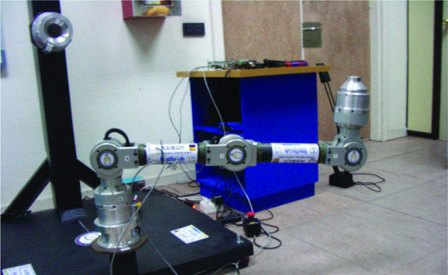
The new method has been implemented in the MATS-ASIBOT platform (see Figure 1 for details). It is a five Degrees of Freedom (DOF) robotic manipulator with 11 kg weight, 1.37 m of maximum reach and it is able to carry a 2 kg payload on each of its two tips. The most important feature of the MATS-ASIBOT platform is that the entire control system is on-board and it only needs a power supply and a wireless user interface from outside. The robot has been conceived as a symmetrical structure which allows it to climb between static and simple docking stations placed into its environment (details in [18]). Additionally, it is equipped with special conical connectors at each of its two tips which allows the robot to perform different movements, as well as the possibility of changing the tip tools in order to perform special tasks or applications [19],[20].

Figure 1.

General view of MATS-ASIBOT with some docking stations.

If two commercial sensors were installed on the robotic platform to obtain force tip measurements (between the wrist and the tool, and between the other wrist and the current docking station), it would be necessary to place on-board (inside the inner volume of the main hollow or in the tubular bars) additional elements which conform to the sensor devices or redesign the structure of the robot. Both options, however, are unfeasible. The method proposed in this work solves the problem of the estimation of the tip forces from both robot tips by placing strain gauges in the two main robot links (bars) and then computing the deflection measurements from the robot structure. Therefore, the robot acts as a flexible structure and the position of the free robot tip is also computed from these measurements because it will be slightly different than the tip position achieved under fully rigid considerations (using kinematic transforms).

The paper is structured as follows: Section 2 is devoted to the modelling of the robot as a flexible structure and presents the model for measuring tip forces adapted to the MATS-ASIBOT platform. The instrumentation system developed is briefly described in Section 3. Experimental results that validate the proposed method are presented in Section 4 and conclusions are stated in Section 5.

2. Main effects of forces over a tip of the robot

2.1 Link flexibility

Figure 2 illustrates all the magnitudes implied in the calculation of the deflection of the whole structure when forces and torques are applied on the nodes of the robot and the flexibility condition is assumed.

Figure 2.

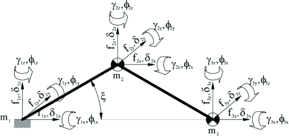
Generalized forces and deflections over the robot.

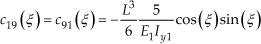
With respect to the base frame and taking into account the symmetry of the structure, the stiffness matrix which relates to the structure displacements regarding the forces applied on the structure can be expressed as a function of the so-called “aperture angle” ξ:

W^{(18 \times 1)} = K^{(18 \times 18)} (ξ) \cdot Δ^{18 \times 1}

(1)

where the vector W denotes the generalized forces and the torques applied on the nodes of the structure, and Δ denotes the linear and the angular deflections of all the nodes. Two important properties of the stiffness matrix are that it is a positive-definite and symmetrical matrix. The inverse relationship between generalized forces and displacements is the compliance matrix which is also ξ-dependant and retains the properties of the stiffness matrix described above. Then,

Δ^{(18 \times 1)} = K^{{(18 \times 18)}^{- 1}} (ξ) \cdot W^{18 \times 1} = C^{(18 \times 18)} (ξ) \cdot W^{18 \times 1}

(2)

Vectors W and Δ are organized according to whether their values are known or unknown as:

\begin{array}{l} \begin{matrix} W = & {(\begin{matrix} W_{k} \\ W_{u} \end{matrix})}^{(12 \times 1 + 6 \times 1)} = & {(\begin{matrix} F_{2}^{T} & Γ_{2}^{T} & F_{3}^{T} & Γ_{3}^{T} & | F_{1}^{T} & Γ_{1}^{T} \end{matrix})}^{T} \end{matrix} \\ \begin{matrix} Δ = & {(\begin{matrix} Δ_{u} \\ Δ_{k} \end{matrix})}^{(12 \times 1 + 6 \times 1)} = & {(\begin{matrix} Δ_{2}^{T} & Φ_{2}^{T} & Δ_{3}^{T} & Φ_{3}^{T} & | Δ_{1}^{T} & Φ_{1}^{T} \end{matrix})}^{T} \end{matrix} \end{array}

(3)

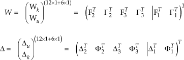
where F_i = (f_ix f_iy f_iz)^T and T_i=(γ_ix γY_iy γ_iz)^T denote the forces and torques on the node ‘i’, while the linear and angular deflections are expressed as Δ_i=(δ_ix δ_iy δ_iz)^T and Φ_i=(φ_ix φ_iy φ_iz)^T for i = 1, 2, 3, respectively. Subscripts ‘u’ and ‘k’ indicate unknown and known parameters. This vector organization lets dispose expression (1) as:

{(\begin{matrix} W_{k} \\ W_{u} \end{matrix})}^{(12 \times 1 + 6 \times 1)} = (\begin{matrix} K_{u u} ​^{12 \times 12} & K_{u k} ​^{12 \times 6} \\ K_{k u} ​^{6 \times 12} & K_{k k} ​^{6 \times 6} \end{matrix}) \cdot {(\begin{matrix} Δ_{u} \\ Δ_{k} \end{matrix})}^{(12 \times 1 + 6 \times 1)}

(4)

The known values of the sub-vector Wk are the corresponding values of node 2 and the values to be measured of node 3, while the known values of Δk are the displacements of the robot base, which are considered null. For the given structure, the following known expanded sub-vectors are used, g being the gravity constant and m2, m3 the lumped masses over nodes 2,3:

\begin{array}{l} W_{k} = \\ = {(\begin{matrix} 0 & 0 & - g m_{2} & 0 & 0 & 0 & f_{3 x} & f_{3 y} & {f_{3 z} - g m_{3}} & 0 & 0 & 0 \end{matrix})}^{T} \end{array}

(5)

Δ_{k} = {(\begin{matrix} \begin{matrix} 0 & 0 & 0 \end{matrix} & \begin{matrix} 0 & 0 & 0 \end{matrix} \end{matrix})}^{T}

(6)

While the reaction forces and the torques on the base and the structure displacements which compose the unknown sub-vectors, Wu and Δu respectively, are computed by adapting expression (4) as:

Δ_{u} = K_{u u} ​^{- 1} \cdot (W_{k} - K_{u k} \cdot Δ_{k})

(7)

W_{u} = K_{k u} \cdot (Δ_{u} + K_{k k} \cdot Δ_{k})

(8)

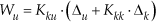
Taking into account that the known displacement sub-vector is null (see equation (6)), the deflections on the whole structure Δ_u and the known forces W_k are obtained from equation (7). Expressions (2) and (7) are rewritten in a reduced size and only K_uu^(12×12) needs to be inverted:

Δ_{u} ​^{(12 \times 1)} = C {(ξ)}^{12 \times 12} = K_{u u}^{- 1} {(ξ)}^{(12 \times 12)} \cdot W_{k} ​^{12 \times 1}

(9)

Due to the symmetry of the structure, all the coefficients of the compliance matrix are obtained as a function of the angle ξ via symbolic methods. If more complex structures (as in [12]) were taken into consideration, the symbolic coefficients could not be achieved and numerical computations and tabulating are required.

The whole compliance matrix has to be computed if all the unknown values have to be estimated. Nevertheless, if only the knowledge of the relation between the forces and the linear displacements is required, a much more reduced compliance matrix can be applied. Under this last assumption, the new reduced matrix is composed of the following coefficients:

C {(ξ)}^{6 x 6} = (\begin{matrix} c_{11} & 0 & c_{13} & c_{17} & 0 & c_{19} \\ 0 & c_{22} & 0 & 0 & c_{28} & 0 \\ c_{13} & 0 & c_{33} & c_{37} & 0 & c_{39} \\ c_{71} & 0 & c_{73} & c_{77} & 0 & c_{79} \\ 0 & c_{82} & 0 & 0 & c_{88} & 0 \\ c_{91} & 0 & c_{93} & c_{97} & 0 & c_{99} \end{matrix})

(10)

Finally, if only the relation between tip forces and tip linear deformations is required (when only a tip lumped mass allows modelling the system), the compliance matrix becomes:

C {(ξ)}^{3 x 3} = (\begin{matrix} c_{77} & 0 & c_{79} \\ 0 & c_{88} & 0 \\ c_{97} & 0 & c_{99} \end{matrix})

(11)

where axial effects have been neglected and only bending and torsion effects are computed:

c_{11} (ξ) = \frac{L^{3}}{3} \frac{1}{E_{1} I_{y 1}} \sin^{2} (ξ)

(12)

c_{13} (ξ) = c_{31} (ξ) = \frac{L^{3}}{3} \frac{1}{E_{1} I_{y 1}} \cos (ξ) \sin (ξ)

(13)

c_{22} (ξ) = \frac{L^{3}}{3} \frac{1}{E_{1} I_{Z 1}}

(14)

c_{33} (ξ) = \frac{L^{3}}{3} \frac{1}{E_{1} I_{y 1}} \cos^{2} (ξ)

(15)

c_{17} (ξ) = c_{71} (ξ) = - \frac{L^{3}}{6} \frac{1}{E_{1} I_{y 1}} \sin^{2} (ξ)

(16)

c_{19} (ξ) = c_{91} (ξ) = - \frac{L^{3}}{6} \frac{5}{E_{1} I_{y 1}} \cos (ξ) \sin (ξ)

(17)

c_{28} (ξ) = c_{82} (ξ) \frac{L^{3}}{6} (\frac{5}{E_{1} I_{z 1}} \cos^{2} (ξ) - \frac{1}{E_{1} I_{z 1}} \sin^{2} (ξ))

(18)

c_{37} (ξ) = c_{73} (ξ) = \frac{L^{3}}{6} \frac{1}{E_{1} I_{y 1}} \cos (ξ) \sin (ξ)

(19)

c_{39} (ξ) = c_{93} (ξ) = \frac{L^{3}}{6} \frac{5}{A_{1} E_{1} I_{y 1}} \cos^{2} (ξ)

(20)

c_{77} (ξ) = \frac{L^{3}}{3} (\frac{1}{E_{1} I_{y 1}} + \frac{1}{E_{2} I_{y 2}}) \sin^{2} (ξ)

(21)

c_{79} (ξ) = c_{97} (ξ) = \frac{L^{3}}{3} (\frac{2}{E_{1} I_{y 1}} + \frac{1}{E_{2} I_{y 2}}) \cos (ξ) \sin (ξ)

(22)

\begin{array}{l} c_{88} (ξ) = \frac{L^{3}}{3} [(\frac{1}{E_{2} I_{z 2}} + \frac{7}{E_{1} I_{z 1}}) \cos^{4} (ξ) + \\ + \frac{L^{3}}{3} (\frac{2}{E_{2} I_{z 2}} + \frac{4}{E_{1} I_{z 1}} + \frac{12}{G_{1} I_{x 1}}) \cos^{2} (ξ) \sin^{2} (ξ) + \\ + \frac{L^{3}}{3} (\frac{1}{E_{2} I_{z 2}} + \frac{1}{E_{1} I_{z 1}}) \sin^{4} (ξ)] \end{array}

(23)

c_{99} (ξ) = \frac{L^{3}}{3} (\frac{7}{E_{1} I_{y 1}} + \frac{1}{E_{2} I_{y 2}}) \cos^{2} (ξ)

(24)

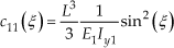
The coefficients showed above are a function of the Young modulus E1, E2, the shear modulus G, the inertia moments of the beams I_1x, I_1y, I_1z, I_2x, I_2y, I_2z and the length L. These coefficients can be simplified if identical beams are used (E₁ = E₂ and I_1x=I_2x, I_1y=I_2y, I_1z=I_2z or I_x = I_y) (see details in [12]).

After obtaining the coefficients of the compliance matrix, expression (9) cannot be solved because the components of the tip forces F₃ are still unknown. The same conclusion is valid for equations (10) and (11) by simple inspection of sub-vector Wk given in equation (5).

Next sub-section shows the model for obtaining the tip forces which are responsible for the deflection of the structure and will allow to measure these forces.

2.2 Joint Torques

Figure 3 shows the main kinematics parameters of the first three DOF of the proposed robot and the involved forces. Due to the symmetry of the robot, the base and the tip are interchangeable nodes (and joints 1,2 are exchanged by joints 5,4), but for the sake of simplicity, node 1 is always considered the fixed one, node 3 represents the mobile tip and the fourth and fifth DOF of the robot are not considered here.

Figure 3.

Main variables of the 3 first DOF of the robot

The main gravitational force effects on m2 results in a flexion of the first link (bar) and a reaction torque on the second joint. This torque is easily computed as:

γ_{2 g} = - L \cdot g \cdot m_{2} \cdot \cos (θ_{2})

(25)

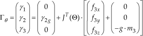
While the effect of any force on the robot tip causes a flexion on the whole structure and reaction torques on the joints, under quasi-static conditions, it is known [3],[4] that the relation between the tip forces and the joint torques is well-determined from the transpose of the geometric Jacobian:

Γ_{θ 3} = J^{T} (Θ) \cdot F_{t i p}

(26)

where Γ_3θ=(γ₁₃γ₂₃γ₃₃)^T and F_tip=F₃+F_3g with F_3g =(0 0 -g·m₃)^T denote the torques on the joint and the tip forces respectively, and Θ=(θ₁ θ₂ θ₃)^T denotes the three first joint angular coordinates. From Figure 3, Denavit-Hartenberg parameters of the first three DOF of the robot are depicted in Table 1:

Table 1.

Denavit-Hartenberg parameters of the first three DOF.

i	θ_i	a_i	α_i
1	θ₁	0	π/2
2	θ₂	L	0
3	θ₃	L	0

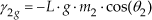
The geometric Jacobian of the reduced robot is obtained from its kinematics parameters as:

J^{T} = (\begin{matrix} - L \cdot s_{1} (c_{2} + c_{23}) & L \cdot c_{1} (c_{2} + c_{23}) & 0 \\ - L \cdot c_{1} (s_{2} + s_{23}) & - L \cdot s_{1} (s_{2} + s_{23}) & L \cdot (c_{2} + c_{23}) \\ - L \cdot c_{1} s_{23} & - L \cdot s_{1} s_{23} & L \cdot c_{23} \end{matrix})

(27)

where c_i=cos(θ_i), s_i= sin(θ_i), c₂₃ = cos(θ₂+θ₃) and s₂₃ = sin(θ₂+θ₃).

Singularities of the reduced robot have to be taken into consideration in order to invert this matrix and their singular joint values can be obtained by solving the following expression:

| J (Θ) | = \det (J {(Θ)}^{T}) = - L^{3} \cdot s_{3} (c_{2} + c_{23}) = 0

(28)

whose solution does not depend on the first joint angle and which allows us to obtain the singular robot configurations

{\begin{matrix} θ_{3} = 0 & o r & θ_{3} = π & ​ & ​ \\ c_{2} + c_{23} = 0 & ​ & ​ & ​ & ​ \end{matrix}

(29)

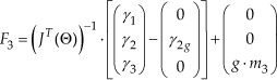
If non-singular postures are considered, the inverse relationship between the join torques and the tip forces is achieved by inverting expression (27):

{(J^{T})}^{- 1} = \frac{1}{L s_{3}} (\begin{matrix} - \frac{s_{1} s_{3}}{(c_{2} + c_{23})} & c_{1} c_{23} & - c_{1} (c_{2} + c_{23}) \\ - \frac{c_{1} c_{3}}{(c_{2} + c_{23})} & s_{1} c_{23} & - s_{1} (c_{2} + c_{23}) \\ 0 & s_{23} & - (s_{2} + s_{23}) \end{matrix})

(30)

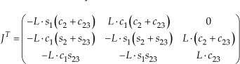
Then, the tip forces together with the gravitational force on m3 are computed from the joint torques as (inverse of equation (26)):

{(\begin{matrix} f_{3 x} & f_{3 y} & {f_{3 z} - g \cdot m_{3}} \end{matrix})}^{T} = {(J^{T} (Θ))}^{- 1} \cdot Γ_{θ 3}

(31)

Finally, from equations (25), (26), (30) and (31) the total joint torques due to the gravitational forces on the structure nodes and due to the tip forces are obtained as:

Γ_{θ} = (\begin{matrix} γ_{1} \\ γ_{2} \\ γ_{3} \end{matrix}) = (\begin{matrix} 0 \\ γ_{2 g} \\ 0 \end{matrix}) + J^{T} (Θ) \cdot [(\begin{matrix} f_{3 x} \\ f_{3 y} \\ f_{3 z} \end{matrix}) + (\begin{matrix} 0 \\ 0 \\ - g \cdot m_{3} \end{matrix})]

(32)

and the external tip forces are obtained as:

F_{3} = {(J^{T} (Θ))}^{- 1} \cdot [(\begin{matrix} γ_{1} \\ γ_{2} \\ γ_{3} \end{matrix}) - (\begin{matrix} 0 \\ γ_{2 g} \\ 0 \end{matrix})] + (\begin{matrix} 0 \\ 0 \\ g \cdot m_{3} \end{matrix})

(33)

3. Instrumentation for tip forces' measurements

Assuming that the robot is a flexible structure composed of two main tubular beams with finite stiffness linked with the three main robot joints which are considered rigid, five strain gauge sets are placed on the two main flexible links of the robot according to Figure 4. Four pairs of 120 Ω Kyowa Strain gauges for sensing bending deformation are located on the bases of both links on opposite sides for each of the orthogonal main directions of these links. Each pair is denoted with under scripts_x1 and_x2. The script x = 1, 2 are for the gauges located at the beginning of the first tube and the scripts x = 4, 5 are for the gauges located at the end of the last tube, while four identical (120 Ω too) gauges are placed to measure the torques on the central joint (denoted with under script_3k with k = 1, 2, 3, 4). They are disposed as indicated in Figure 4 at the end of the first tube together with the beginning of the second one. Only the sets with x = 1, 2 and 3 are employed for the experiments and only sets with x = 5, 4 and 3 would be employed if the tip and the base were exchanged.

All gauge pairs use ½ Wheatstone bridge-based amplifiers except gauge set 3 which uses a full bridge configuration with a 4-active-guage system. Simpler configurations can be defined, but the same number of bridges is needed. Single gauges can be employed for any of the main directions of each of the links (orthogonally disposed) and only a ¼ bridge is needed to measure the deflections. Temperature compensation has to be taken into consideration for accuracy measurements.

Figure 4.

Location of the strain gauges over the flexible tubes.

The ±10 V signal output from the amplifiers are acquired through on-board AD converters. From these voltage values and by real-time computation of the compliance and the Jacobian matrices, the variation in the gauge resistor allows us to measure the joint torques produced by the forces on the robot and to obtain the deflection of the structure.

4. Experimental results

A general view of the MATS-ASIBOT was depicted in Figure 1 when it was disposed in a vertical pose and connected to one of the docking stations (resting posture of the robot). Additionally, in Figure 1, we can see four docking stations (with different positions and orientations) disposed on a metallic support station.

In this section, three experiments were carried out using the MATS-ASIBOT setup. All the experiments were performed following a similar procedure, i.e., the robot starts the motion from its resting posture and finishes its motion in one of the three different final selected postures or returning to the initial posture. Different forces appear on the robot during its movement: gravitational forces are only considered in the two first experiments, while in the third experiment the robot interacts with the environment causing not only gravitational but also external tip forces.

4.1 Free motion with non-singular postures

The first experiment begins with moving the robot from the resting posture P₀ (see Figure 1) to the final posture P_f₁ (see Figure 5). Gravitational forces act on the masses m2 and m3. Figure 6 illustrates several intermediate postures with the robot assumed rigid – plotted in red colour – and the robot with the added flexibility effects –green colour – (units in cm). The deformed representations of the structure have been computed by using the reduced compliance matrix given in expression (10) and the coefficients expressed in (12)–(24). Point-to-Point trajectories with trapezoidal velocity profiles were used. In this first case, the joint trajectories were generated from next joint coordinates and t₀ = 10, t_f = 25s:

(\begin{matrix} θ_{10} = 0 \\ θ_{20} = π ∕ 2 \\ θ_{30} = 0 \end{matrix}) \overset{t o}{\to} (\begin{matrix} θ_{1 f 1} = 0 \\ θ_{2 f 1} = 0 \\ θ_{3 f 1} = π ∕ 2 \end{matrix}) rad

(34)

Figure 5.

Final posture Pf1 selected in the first experiment.

Figure 6.

Some rigid and flexible postures from P0 to Pf1.

Using equation (32) for the final robot posture in the first experiment, the following relation between the tip forces and the join torques is achieved as

(\begin{matrix} γ_{1} \\ γ_{2} \\ γ_{3} \end{matrix}) = (\begin{matrix} 0 \\ - g \cdot L \cdot m_{2} \\ 0 \end{matrix}) + (\begin{matrix} 0 & L & 0 \\ - L & 0 & L \\ - L & 0 & 0 \end{matrix}) \cdot (\begin{matrix} f_{3 x} \\ f_{3 y} \\ f_{3 z} - g \cdot m_{3} \end{matrix})

(35)

Figure 7 plots the measured torque γ₂(t) (thin blue) compared to the estimated torque γ_{2_Estimated}(t) (thick red) which is computed from equation (32) under the assumption that only gravitational forces act on the robot during the movement.

Figure 7.

Torque γ₂ during trajectory from P₀ to P_f1.

The lengths of the main links L = 0.6685 m are defined as the distances between joints 2-3-4. Furthermore, the values of the lumped masses have been fitted to the values expressed in (36) after using the least-squared methods and identifying them as a two lumped masses model. Remember that one of the masses (m1 or m3) is always fixed to one of the docking stations (exchangeable nodes). In the experiment m1 is considered the fixed node.

{\begin{matrix} m_{1} = & 4.27 & k g \\ m_{2} = & 2.46 & k g \\ m_{3} = & 4.27 & k g \end{matrix}

(36)

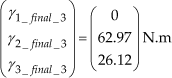
Operating with equation (35) and (36), the steady state final values of the joint torques are:

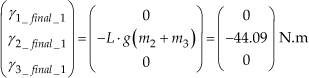
(\begin{matrix} γ_{1_f i n a l_1} \\ γ_{2_f i n a l_1} \\ γ_{3_f i n a l_1} \end{matrix}) = (\begin{matrix} 0 \\ - L \cdot g (m_{2} + m_{3}) \\ 0 \end{matrix}) = (\begin{matrix} 0 \\ - 44.09 \\ 0 \end{matrix}) N .m

(37)

Figure 8 depicts the measured torques γ₁(t) and γ₃(t) versus the null desired values expressed in (32) and final values achieved in (37).

Figure 8.

Torques γ₁, γ₃ during trajectory from P₀ to P_f1.

From the first final robot posture, and according to equation (33), the tip forces are computed as:

(\begin{matrix} f_{3 x_e s} \\ f_{3 y_e s} \\ f_{3 z_e s} \end{matrix}) = \frac{1}{L} (\begin{matrix} 0 & 0 & - 1 \\ 1 & 0 & 0 \\ 0 & 1 & - 1 \end{matrix}) \cdot [(\begin{matrix} γ_{1 m} \\ γ_{2 m} \\ γ_{3 m} \end{matrix}) + (\begin{matrix} 0 \\ L \cdot g \cdot m_{2} \\ 0 \end{matrix})] + (\begin{matrix} 0 \\ 0 \\ g \cdot m_{3} \end{matrix})

(38)

Computing the average values of the steady state final measured torques depicted in Figures 7 and 8, and replacing them into equation (37), yields:

(\begin{matrix} f_{3 x_e s} \\ f_{3 y_e s} \\ f_{3 z_e s} \end{matrix}) = \frac{1}{0.6685} (\begin{matrix} 0 & 0 & - 1 \\ 1 & 0 & 0 \\ 0 & 1 & - 1 \end{matrix}) \cdot [(\begin{matrix} - 1.9 \\ - 44.2 \\ - 2.4 \end{matrix}) + (\begin{matrix} 0 \\ 16.1 \\ 0 \end{matrix})] + (\begin{matrix} 0 \\ 0 \\ 41.8 \end{matrix})

(39)

The estimation of the tip forces applied in this experiment were F₃^T=(3.59 2.84 0.23V N showing good correspondence between the measured and the estimated values. Moreover, we can see how the low resolution of the used converters makes the estimation of the tip forces not so good for components f_3x and f_3y near zero values. The error achieved from f_3z is considered an acceptable error. The use of AD converters with more number of bits and a computer-based method for placing the gauges over the structure allow increasing the resolution of the system and reducing the observed errors.

4.2 Free motion with singular postures

The second experiment starts moving the robot from the resting posture (see Figure 1) to the new final posture P_f2 (see Figure 9). Figure 10 depicts several intermediate postures with the robot assumed rigid and including the additional flexibility effects due to the gravitational forces on m2 and m3 (units in cm). Point-to-Point trajectories with trapezoidal velocity profiles were used from next joint coordinates with the same max velocity as in the previous experiment:

(\begin{matrix} θ_{10} = 0 \\ θ_{20} = π ∕ 2 \\ θ_{30} = 0 \end{matrix}) \overset{t o}{\to} (\begin{matrix} θ_{1 f 2} = 0 \\ θ_{2 f 2} = 0 \\ θ_{3 f 2} = 0 \end{matrix}) rad

(40)

Figure 9.

Second final robot posture P_f2.

Figure 10.

Some rigid and flexible postures from P₀ to P_f2.

If the second final posture P_f₂ is considered, regardless to the movement of the fourth and fifth joint, it can clearly be seen that all postures correspond with singular robot points and the Jacobian matrix becomes not invertible(θ₂=0). Then, for the final posture P_f₂, the relation between tip forces and joint torques is given by:

(\begin{matrix} γ_{1} \\ γ_{2} \\ γ_{3} \end{matrix}) = (\begin{matrix} 0 \\ - L \cdot g \cdot m_{2} \\ 0 \end{matrix}) + (\begin{matrix} 0 & 2 L & 0 \\ 0 & 0 & 2 L \\ 0 & 0 & L \end{matrix}) \cdot (\begin{matrix} f_{x} \\ f_{y} \\ f_{z} - g \cdot m_{3} \end{matrix})

(41)

Following a similar procedure as in the previous experiment, Figure 11 plots the measured torque γ₂(t) versus the estimated torque γ_{2_Estimated}(t) which is computed from equation (32) under the assumption that only gravitational forces act on the robot during the movement.

Figure 11.

Torques γ₂, γ₃ during trajectory from P₀ to P_f2.

From equations (41) and (36), the steady state final values of the joint torques are as follows:

(\begin{matrix} γ_{1_f i n a l_2} \\ γ_{2_f i n a l_2} \\ γ_{3_f i n a l_2} \end{matrix}) = (\begin{matrix} 0 \\ - L \cdot g (m_{2} + 2 m_{3}) \\ - L \cdot g \cdot m_{3} \end{matrix}) = (\begin{matrix} 0 \\ - 72.13 \\ - 27.97 \end{matrix}) N m

(42)

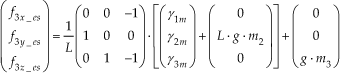
For the second final robot posture, the tip forces have to be computed by using a pseudo-inverse matrix under the assumptions that the force f_3x does not produce any structure torque and the traction on the tubular beams has been fully neglected in coefficients (12)–(24). Then, equation (33) becomes:

(\begin{matrix} 0 \\ f_{3 y_e s} \\ f_{3 z_e s} \end{matrix}) = \frac{1}{L} (\begin{matrix} 0 & 0 & 0 \\ 0.5 & 0 & 0 \\ 0 & 0.5 & 0 \end{matrix}) [(\begin{matrix} γ_{1 m} \\ γ_{2 m} \\ γ_{3 m} \end{matrix}) + (\begin{matrix} 0 \\ L \cdot g \cdot m_{2} \\ 0 \end{matrix})] + (\begin{matrix} 0 \\ 0 \\ g \cdot m_{3} \end{matrix})

(43)

Again, computing the average values of the steady state final measured torques from the signals plotted in Figure 11 and substituting them into equation (43), yields:

(\begin{matrix} 0 \\ f_{3 y_e s} \\ f_{3 z_e s} \end{matrix}) = \frac{1}{0.6685} (\begin{matrix} 0 & 0 & 0 \\ 0.5 & 0 & 0 \\ 0 & 0.5 & 0 \end{matrix}) [(\begin{matrix} 1.6 \\ - 71.9 \\ - 27.4 \end{matrix}) + (\begin{matrix} 0 \\ 16.1 \\ 0 \end{matrix})] + (\begin{matrix} 0 \\ 0 \\ 41.8 \end{matrix})

(44)

The external tip forces were estimated again, being F₃ ^T = (0 1.20 0.29)^T N, showing a good correspondence between the measured and the estimated values. These errors are due to the low resolution of the AD converters used and they are less than 1/2n, n being the number of bits. Additionally, because of the singularity of the robot postures during the experiment, the average steady-state torque γ₃ shown in Figure 11 is not involved in the computation of the tip force due to the last zero column of the pseudo-inverse matrix. A good correspondence is also observed between this value and the expected value achieved from expression (42).

4.3 Free motion with final object interaction

In this experiment, the robot starts its motion from the resting posture (Figure 1) to the final posture P_f₃(see in Figure 12). Then, it returns to the resting posture after pressing an object. In this case the contact with the object produces a tip force which is coupled with the gravitational forces applied to the robot during the motion. The first three joint trajectories are generated from the following joint coordinates:

(\begin{matrix} θ_{10} = 0 \\ θ_{20} = π ∕ 2 \\ θ_{30} = 0 \end{matrix}) \overset{t o}{\to} (\begin{matrix} θ_{1 f 3} = 0 \\ θ_{2 f 3} = 2.609 \\ θ_{3 f 3} = 0.899 \end{matrix}) \overset{t o}{\to} (\begin{matrix} θ_{10} = 0 \\ θ_{20} = π ∕ 2 \\ θ_{30} = 0 \end{matrix}) rad

(45)

Figure 12.

Final posture P_f3 when the robot interacts with a box.

Figure 13 depicts several intermediate postures during the free robot motion under the assumption that the robot is rigid and including the additional flexibility effects due to the gravitational forces on m2 and m3 (units in cm). It can clearly be seen how the flexible robot reaches the final posture before the rigid robot does because of these gravitational forces for the same joint coordinates. The plotted deflections have been intentionally exaggerated.

Figure 13.

Some rigid and flexible postures from P₀ to P_f3.

Once the robot (assumed flexible) has reached the real final posture, a contact force is applied on its tip. The robot is now pressing the box and Figure 14 represents how the robot flexion turns over the opposite sign compared to the flexion depicted in the same final posture (see Figure 13) when the robot was moving freely.

Figure 14.

Rigid and flexible robot when pressing the box.

Finally, applying equation (32) again for the P_f₃posture without external tip forces, the steady state final measured torque values computed are as follows:

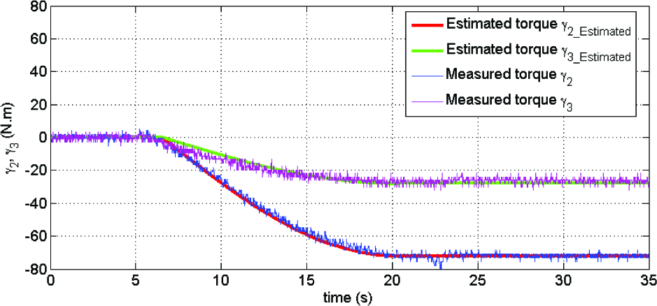
(\begin{matrix} γ_{1_f i n a l_3} \\ γ_{2_f i n a l_3} \\ γ_{3_f i n a l_3} \end{matrix}) = (\begin{matrix} 0 \\ 62.97 \\ 26.12 \end{matrix}) N .m

(46)

Figures 15 and 16 illustrate the measured torques, γ₂(t) and γ₃(t), of this experiment versus the estimated values of the torques caused from the gravitational forces.

Figure 15.

Torque γ₂ during trajectory from P₀ P_f3 P₀ and the interaction with the box.

Figure 16.

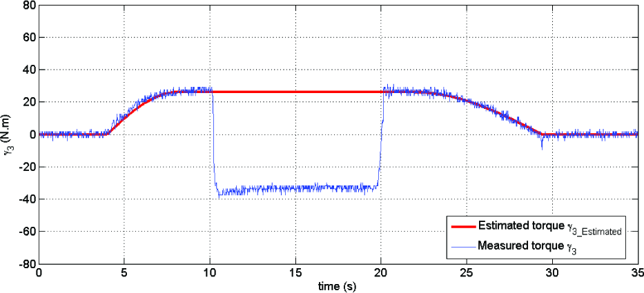
Torque γ₃ during trajectory from P₀-P_f3-P₀ and the interaction with the box.

The time interval can also be seen while the robot is pressing the box (between t = 10 s and t = 20 s) and when estimation of the torques due to gravity does not match real torques. This difference between estimated and measured torques anticipates that some external forces are being applied on the tip and it can also be used as a contact/collision indicator (as in [21]).

By using equation (33), which requires the online computation of the torques due to gravity and the inverse of the Jacobian transpose as a function of its joint coordinates, let us obtain the applied forces. Figure 17 depicts the tip force component f_3z obtained. Components f_3x and f_3y are not plotted due to their good match with noisy null values. The values of the external tip forces during the free movement of the robot are also plotted in Figure 17 (in red colour).

Figure 17.

Tip force f_3z during interaction with the box.

It is necessary to remark that the noise levels of these signals are typical from strain measurements when no low-pass filters are used. All the figures have been plotted with the values directly obtained from the AD converters and without any kind of filter. Once the system is calibrated, only easy algebraic operations and scaling matrix according to the equations presented above have been used to achieve the previous results.

5. Conclusions

A method to measure external forces applied on the tip of a climbing robot whose structure exhibits linear flexibility has been presented. The main advantage is the elimination of the usual force sensors placed between the wrists and tools in industrial robotics applications that require force or hybrid position/force controllers.

The placement of strain gauges along the structure allows us to measure deflections from the structure itself. The torques produced on the robot flexible structure are obtained from the strain gauges and the forces are computed. It is necessary to estimate gravity torques in order to discount them from the total measured torques if only external forces are required to be measured.

The use of strain gauges instead of force sensors has the following advantages: (a) the use of flexible elements can be exploited for lightening the links/legs that conform to different locomotion systems which make up climbing robots, and (b) the flexibility of the structure is used to measure the tips forces applied and only a set of strain gauges with electronic conditioners and AD converters is needed for acquisition. From these force measurements, the structure deflection itself is computed through the compliance matrix which is dependent on the joint angles.

Experimental results illustrate the robustness of the proposed method when only the gravitational forces act on a robot with flexibility that could be modelled as a lumped mass model and when it is working under difficult trajectories such as trajectories with kinematics singularities. When not only gravitational forces but external ones were applied on the robot tip, the proposed method let us obtain the forces as if it were a sensor.

Footnotes

6. Acknowledgments

Prof. Somolinos wishes to thank the faculty and staff of the Robotics Lab at the University Carlos III of Madrid for their excellent reception during his stay which allowed the realization of this work. It has been partially supported by Spanish Research Grant DPI2011-24113.

References

Ati Industrial Automation. Multi-Axis Force/Torque Sensors. www.ati-ia.com/products/ft/sensors.aspx.

Scheinman

. (1969) Design of a computer controlled manipulator. Ph.D. Thesis. Stanford University.

Craig

. (1989) Introduction to Robotics. Mechanics and Control. Second Edition. Addison-Wesley.

Sciavicco

Siciliano

(2000) Modelling and Control of Robot Manipulators. Springer Verlag. London UK.

Mallapragada

Erol

Sarkar

(2007) A New Method of Force Control for Unknown Environments International Journal of Advanced Robotic Systems, Vol. 4, No. 3, pp. 313–322.

Wen

Zheng

Zhu

and Chen

(2012) Elman Fuzzy Adaptive Control for Obstacle Avoidance of Mobile Robots Using Hybrid Force/Position Incorporation IEEE Transactions on Systems, Man, and Cybernetics – Part C: Applications and Reviews. Vol. 42, No, 4. pp 603–608.

Chen

. (2012) Kalman Filter for Robot Vision IEEE Transactions on Industrial Electronics. Vol. 59, No, 11. pp 4409–4420.

Mostafa

Tsai

C.S

Her

(2010) Alternative Gaits for Multiped Robots with Leg Failures To Retain Maneuverability International Journal of Advanced Robotic Systems, Vol. 7, No. 4 31, pp. 33–40.

Nickols

(2009) A Tabular Format for Computing Inverse Kinematics Equations for a 3DOF Robot Leg. International Journal of Advanced Robotic Systems, Vol. 6, No. 3, pp. 177–200.

10.

Cao

Zhu

(2011) Dynamic Simulation of Hybrid-driven Planar Five-bar Parallel Mechanism Based on SimMechanics and Tracking Control. International Journal of Advanced Robotic Systems, Vol. 8, No. 4, pp. 28–33.

11.

Asif

U Umar

Iqbal

(2011) Motion Planning Using an Impact-Based Hybrid Control for Trajectory Generation in Adaptive Walking Control. International Journal of Advanced Robotic Systems, Vol. 8, No. 4, pp. 212–224.

12.

Somolinos

Feliu

Sánchez

(2002) Design, Dynamic Modeling and Experimental Validation of a New Three-degrees-of-freedom Flexible Arm. Mechatronics. Vol. 12, No. 7, pp. 919–948.

13.

Thatte

Parness

. (2011) Design of a Robotic Ankle Joint for a Microspine-Based Robot. JPL-NASA USRP - Internship Final Report, pp. 1–7.

14.

Feliu

Payo

Becedas

(2011) Two-Flexible-Fingers Gripper Force Feedback Control System for its Application as End Effector on a 6DOF Manipulator IEEE Transactions on Robotics, Vol. 27, No. 3, pp. 599–615.

15.

Whitesides

. (2011) Freaky Boneless Robot Walks on Soft Legs Freaky Boneless Robot Walks on Soft Legs. IEEE Spectrum March, 29 2011 http://spectrum.ieee.org/automaton/robotics/military-robots/freaky-boneless-robot-walks-on-soft-legs.

16.

Feliu

García

Somolinos

. (2003) Gauge Based Tip Position Control of a new Three degree-of-freedom Flexible Robot. Journal of Robotics Research. Vol. 20, N.8. pp. 660–675.

17.

Somolinos

Morales

Morón

García

(2012) Using the Own Flexibility of a Climbing Robot as a Double Force Sensor. Key Engineering Materials Vol. 495, pp. 91–95.

18.

Balaguer

Giménez

Jardón

(2006) The MATS Robot: Service climbing robot for personal assistance. IEEE Robotics & Automation Magazine. Vol. 13, No. 1, pp. 51–58.

19.

Cabas

Balaguer

(2005) Design and development of a light weight embodied robotic hand activated with only one actuator International Conference on Intelligent Robots and Systems, pp. 2369–2374.

20.

Jardon

(2008). Asibot: Robot portátil de asistencia a discapacitados. Concepto, arquitectura de control y evaluación clínica. Revista Iberoamericana de Automática e Informática Industrial. Vol. 5, No. 2, pp 48–59 (in Spanish).

21.

Feliu

García

Somolinos

. (2003) Experimental Testing of a Gauge Based Collision Detection Mechanism for a new 3DOF Flexible Robot Journal of Robotics Systems. Vol. 20, No, 6. pp 271–283.

Force Sensor of a Climbing Robot Derived from Its Own Flexible Structure

Abstract

Keywords

1. Introduction

2. Main effects of forces over a tip of the robot

2.1 Link flexibility

2.2 Joint Torques

3. Instrumentation for tip forces' measurements

4. Experimental results

4.1 Free motion with non-singular postures

4.2 Free motion with singular postures

4.3 Free motion with final object interaction

5. Conclusions

Footnotes

6. Acknowledgments

References