Uncalibrated Neuro-Visual Servoing Control for Multiple Robot Arms

Abstract

Diverse image-based tracking schemes for a robot moving in free motion have been proposed and experimentally validated. However, few visual servoing schemes have addressed the tracking of the desired trajectory and the contact forces for multiple robot arms. The main difficulty stems from the fact that camera information cannot be used to drive force trajectories. Recognizing this fact, a unique error manifold that includes position-velocity and force errors in orthogonal complements is proposed. A synergistic scheme that fuses camera, encoder and force sensor signals into a unique error manifold allows proposing a control system which guarantees exponential tracking errors under parametric uncertainty. Additionally a small neural network driven by a second order sliding mode surface is derived to compensate robot dynamics. Residual errors that arise because of the finite size of the neural network are compensated via an orthogonalized second order sliding mode. The performance of the proposed scheme, in two significant applications of the multiple robot arms, is validated through numerical simulations.

1. Introduction

To increase the executing tasks of the robot manipulators in several practical applications, the use of multiple robot arms working together in the same workspace and cooperatively has been proposed. Working abilities, loading capabilities and object manipulation are some advantages of multiple robot arms with respect to a single robot. In order to resolve the complex dynamic interactions in these robotic systems, many studies have focused attention on designing robust and adaptive control schemes to minimize the hardware and software.

Although several approaches for cooperative schemes [9, 13, 15], fast control [5, 8, 14, 26], load distribution and path planning [19] have been reported in the literature, a difficultly in synthesizing these approaches in practice is the inexact knowledge of almost all system parameters.

Additionally, to avoid the computational load and the ill-posed nature on the inverse kinematics in the joint robot control, controllers in operational coordinates or the use of visual information called visual servoing can be addressed as an alternative solution.

Despite the fact that several pieces of research have addressed vision/force control [1, 4, 7, 27] for a single robot, few of them show robustness to uncertainties in robot parameters or camera parameters. In [27] a controller based on the multisensor fusion is proposed where the signals from sensors are used to correct uncalibrated parameters. But the force/position controller and the planner require an exact knowledge of the robot manipulator. An adaptive algorithm is used in [21, 22] to estimate the visual Jacobian matrix in free motion. This approach is based on the assumption that the visual Jacobian matrix can be decomposed as a product of two matrices. The first matrix requires kinematic parameters of the robot manipulator, while the second matrix is assumed unknown. That is, the rotation matrix between the robot base frame with respect to the vision frame is unknown. On the other hand, a neurovisual servoing control of a planar robot manipulator is presented in [23] where it is assumed that the link lengths of the robot manipulator are not exactly known. The neural network is used to avoid the drift in the parameter estimated and some possible overshoot in the estimated of the gravitational vector. That is, it is not necessary to know the gravity vector and boundedness of the Jacobian matrix against a perturbation. At the same time, there is a dearth of research that extends or combines these visual approaches to multiple robot arms under parametric uncertainty.

This paper aims to design a theoretical neuro-visual servoing controller that guarantees analytically image-based tracking of constrained multiple robot arms subject to parametric uncertainty, that is, i-th robot and the camera parameters are unknown. The neuro-visual servoing control is based on a second order sliding surface for visual position and contact force trajectories respectively. To approximate the i-th robot dynamics and the parameter variations, a small neural network driven by the sliding mode is used. The residual error that arises from this bounded approximation is eliminated with the sliding mode into a unique error manifold. In contrast with other approaches, in this paper exponential convergence of image-based position error and contact forces are guaranteed with smooth control and chattering free. Finally, the parametric uncertainty on the i-th robot manipulator and camera are parameterized in terms of the regressor time as a parameter vector. Then, to get parametric uncertainty, this vector is multiplied by a factor with respect to the nominal value.

The viability of this approach is demonstrated through two typical applications of the multiple robot manipulators in a horizontal plane. In the first simulation, a pair of robot manipulators grasps an object firmly applying the desired force through the contact point, while the end-effector of the i-th robot manipulator follows the desired visual trajectory. In the second simulation a more complex task is presented, one that involves the changing dynamics and an impact regime to manipulate an object by two robotic fingers. Strictly speaking, transition tasks involve free motion, impact and constrained motion regimes. Impulsive and unilateral constraints arise in the impact regime, which makes it very difficult to design a control system. The simple approach would be to avoid impact and to commute consistently between a free and constrained controller. That is, given that algebraic constraints arise in the constrained regime, a virtual constraint will be proposed to model a DAE1 system for all regimes. Thus, the control scheme proposed is based on the avoiding impact regime, through zero transition velocity from free to constrained motion, which means that impulsive dynamics does not appear. Differently then [18, 24, 25], this approach is one of fast constrained object manoeuvring for non-redundant multiple robot arms. Furthermore, a decentralized cooperative tracking is obtained without using the model of the robot manipulator, nor exact knowledge of the inverse Jacobian.

2. Constrained dynamics of a multiple arms robot

Dynamical Equations. Consider a robotic system composed of l rigid robot manipulators that is holding an object, the differential algebraic dynamic model of the i-th manipulator, i ∊ {1,‥‥,l}, constrained by the object's geometry can be expressed by

$${{\rm H}}_{\mathrm{i}}\left(q_{\mathrm{i}}\right){\ddot{q}}_{\mathrm{i}}+C_{\mathrm{i}}\left(q_{\mathrm{i},}{\dot{q}}_{\mathrm{i}}\right){\dot{q}}_{\mathrm{i}}+g_{\mathrm{i}}\left(q_{\mathrm{i}}\right)=u_{\mathrm{i}}+J_{{\phi }_{\mathrm{i}+}}^{\mathrm{T}}\left(q_{\mathrm{i}}\right){\lambda }_{\mathrm{i}}$$

(1)

$${\phi }_{\mathrm{i}}\left(q_{\mathrm{i}}\right)=0$$

(2)

where $q_{\mathrm{i}},{\dot{q}}_{\mathrm{i}},{\ddot{q}}_{\mathrm{i}}∊{\Re }^{{\mathrm{n}}_{\mathrm{i}}}$ are angular positions, velocities and accelerations of the revolute joints of the i-th manipulator, which has n_i degrees of freedom, $H_{\mathrm{i}}(q_{\mathrm{i}})∊{\Re }^{{\mathrm{n}}_{\mathrm{i}}\times {\mathrm{n}}_{\mathrm{i}}}$ is a positive-definite inertial matrix, $C_{\mathrm{i}}(q_{\mathrm{i}},{\dot{q}}_{\mathrm{i}})∊{\Re }^{{\mathrm{n}}_{\mathrm{i}}\times {\mathrm{n}}_{\mathrm{i}}}$ is a Coriolis matrix which models centripetal and centrifugal forces, $g_{\mathrm{i}}(q_{\mathrm{i}})∊{\Re }^{{\mathrm{n}}_{\mathrm{i}}}$ is a vector of gravitational torques, and $u_{\mathrm{i}}∊{\Re }^{{\mathrm{n}}_{\mathrm{i}}}$ is a vector of input-controlled joint torques. If the end-effector of the i-th robot manipulator is in touch with the frictionless and infinitely rigid surface of the object, which is modelled by the geometric function ${\phi }_{\mathrm{i}}(q_{\mathrm{i}}):{\Re }^{{\mathrm{n}}_{\mathrm{i}}}\to {\Re }^{{\mathrm{m}}_{\mathrm{i}}}$ with m_i > 0 representing the number of independent contact points of the i-th manipulator, then

$$\begin{array}{l}{J}_{\phi }{}_{{}_{\mathrm{i}}}\left(q_{\mathrm{i}}\right)=\nabla {\phi }_{\mathrm{i}}\\ J_{\phi }{}_{{}_{\mathrm{i}+}}\left(q_{\mathrm{i}}\right)=J_{{\phi }_{\mathrm{i}}}^{\mathrm{T}}\left(q_{\mathrm{i}}\right){\left(J_{\phi }{}_{{}_{\mathrm{i}}}\left(q_{\mathrm{i}}\right)J_{{\phi }_{\mathrm{i}}}^{\mathrm{T}}\left(q_{\mathrm{i}}\right)\right)}^{-1}\end{array}$$

where $J_{\phi }{}_{{}_{\mathrm{i}}}(q_{\mathrm{i}})∊{\Re }^{{\mathrm{m}}_{\mathrm{i}}}{}^{\times {\mathrm{n}}_{\mathrm{i}}}$ is the constraint Jacobian, $J_{\phi }{}_{\mathrm{i}+}(q_{\mathrm{i}})∊{\Re }^{{\mathrm{m}}_{\mathrm{i}}}{}^{\times {\mathrm{n}}_{\mathrm{i}}}$ is an orthonormal matrix, and ${\lambda }_{\mathrm{i}}∊{\Re }^{{\mathrm{m}}_{\mathrm{i}}}$ a Lagrange multiplier that represents the magnitude of the contact force.

Manipulation Space. When the robotic system manipulates an object, the position of the i-th end effector is geometrically constrained on a p_i = n_i – m_i dimensional manifold O_ri, where

$${\mathrm{O}}_{\mathrm{r}}{}_{\mathrm{i}}=\{(q_{\mathrm{i}},{\dot{q}}_{\mathrm{i}}):{\phi }_{\mathrm{i}}\left(q_{\mathrm{i}}\right)=0,{\dot{\phi }}_{\mathrm{i}}\left(q_{\mathrm{i}}\right)=0\}$$

From the standpoint of path planning, equation (2) stands for the trajectory to be followed which runs on the surface of the object. Thus, the constraint imposed by equation (2) should be satisfied in all time which means that the manipulator does not invade the object's space.

Even though the formalism presented through the paper can be extended for a i-th rigid manipulator, this work will focus in a robotic system with two manipulators (i = 2), each of them having a single contact point (m_i = 1, for i ∊ {1,2}). This is a planar robotic system, thus the manipulators move in a horizontal plane.

Open Loop Error Equation. According to the properties of equation (1), which can be parametrized linearly [10], in terms of a nominal reference ${\left({\dot{q}}_{ri},{\ddot{q}}_{ri}\right)}^{\mathrm{T}}∊{\Re }^{2n_i}$ as follows

$$H_{\mathrm{i}}\left(q_{\mathrm{i}}\right){\ddot{q}}_{\mathrm{r}\mathrm{i}}+C_{\mathrm{i}}(q_{\mathrm{i}},{\dot{q}}_{\mathrm{i}}){\dot{q}}_{\mathrm{r}\mathrm{i}}+g_{\mathrm{i}}\left(q_{\mathrm{i}}\right)=Y_{\mathrm{r}\mathrm{i}}{\mathrm{m}}_{\mathrm{i}}$$

(3)

where the regressor

$$Y_{\mathrm{r}\mathrm{i}}=Y_{\mathrm{r}\mathrm{i}}\left(q_{\mathrm{i}},{\dot{q}}_{\mathrm{i},}{\dot{q}}_{\mathrm{r}\mathrm{i},}{\ddot{q}}_{\mathrm{r}\mathrm{i}}\right)∊{\Re }^{{\mathrm{n}}_{\mathrm{i}}\times {\mathrm{n}}_{\mathrm{i}}}$$

is composed of known non-linear functions, and m_i ∊ ℜ^pi represents unknown but constant parameters. If we add and subtract equation (3) to equation (1), then the following open loop error equation arises

$$H_{\mathrm{i}}\left(q_{\mathrm{i}}\right){\dot{s}}_{\mathrm{i}}+C_{\mathrm{i}}\left(q_{\mathrm{i}},{\dot{q}}_{\mathrm{i}}\right)s_{\mathrm{i}}=u_{\mathrm{i}}+\text{}{J}_{{\phi }_{\mathrm{i}+}}^{\mathrm{T}}\left(q_{\mathrm{i}}\right){\lambda }_{\mathrm{i}}-Y_{\mathrm{r}\mathrm{i}}{\mathrm{m}}_{\mathrm{i}}$$

(4)

where the joint error manifold is defined by

$$s_{\mathrm{i}}={\dot{q}}_{\mathrm{i}}-{\dot{q}}_{\mathrm{r}\mathrm{i}}$$

(5)

Constrained Positions and Velocities. Once the manipulators jointly grasp an object and hold it securely, they keep pulling and pushing. Thus, in order to work in a cooperative manner and to rigidly manipulate an object, we need to model these effects. This is achieved by using constrained position and constrained velocity variables [14]. Considering the total derivative of the holonomic constraints imposed by equation (2), the constrained position and constrained velocity are defined as

$$p_{\mathrm{i}}={\displaystyle \sum _{\mathrm{j}=1}^{\mathrm{l}}{\displaystyle {\int }_{\mathrm{t}\mathrm{o}}^{\mathrm{t}\mathrm{f}}{J}_{{\phi }_{\mathrm{j}}}\left(q_{\mathrm{j}}\right){\dot{q}}_{\mathrm{j}}\mathrm{d}\mathrm{t}}},{\dot{p}}_{\mathrm{i}}={\displaystyle \sum _{\mathrm{j}=1}^{\mathrm{l}}{J}_{{\phi }_{\mathrm{j}}}}\left(q_{\mathrm{j}}\right){\dot{q}}_{\mathrm{j}}$$

(6)

respectively. Consequently, to propose an appropriate error coordinate system, equation (6) should be included in the error manifold through ${\dot{q}}_{\mathrm{r}\mathrm{i}}.$ .

In order to design an image-based decentralized controller without resorting to $H_{\mathrm{i}}(q_{\mathrm{i}}),C_{\mathrm{i}}(q_{\mathrm{i}},{\dot{q}}_{\mathrm{i}})$ and g_i(q_i), we need to define a joint error manifold that uses the visual position of the CCD camera sensor. Firstly, let us establish a mapping between joint velocities and end-effector visual velocities.

Visual Kinematics. Let the direct and differential kinematics for the i-th robot manipulator be defined by

$$\begin{array}{l}{x}_{\mathrm{b}}{}_{{}_{\mathrm{i}}}=f_{\mathrm{i}}\left(q_{\mathrm{i}}\right)\\ {\dot{x}}_{{\mathrm{b}}_{\mathrm{i}}}=J_{\mathrm{i}}\left(q_{\mathrm{i}}\right){\dot{q}}_{\mathrm{i}}\end{array}$$

(7)

where f_i:ℜⁿ → ℜⁿ is the generally non-linear forward kinematics, $x_{b_i}∊{\Re }^{\mathrm{n}}$ represents the end-effector position of the i-th robot manipulator in the operational workspace, and J_i(q_i) its Jacobian matrix. Given that a planar robot is used in this work, the operational space has two dimensions and n = 2. In this paper we use a widely accepted fixed (static) camera configuration [6], which has a thin lens without aberration, whose mathematical description consists of a composition of four transformations that take into account: joint to Cartesian transformation, Cartesian to camera transformation, camera to CCD transformation, and CCD to image transformation. Therefore, the 2D visual position $x_{s_i}∊{\Re }^2$ of the CCD camera sensor, which maps the i-th end-effector position into the image space (screen), is given by

$$x_{s_i}=\alpha R{x}_{\mathrm{b}\mathrm{i}}+b$$

(8)

with

$$\begin{array}{l}\alpha ={\alpha }_0\frac{{\lambda }_{\mathrm{f}}}{{\lambda }_{\mathrm{f}}-\mathrm{z}},R=\left[\begin{array}{cc}\cos \left(\theta \right)& -\sin \left(\theta \right)\\ \sin \left(\theta \right)& \cos (\theta )\end{array}\right]\\ \mathrm{a}\mathrm{n}\mathrm{d}b\mathrm{ }={\alpha }_0\frac{{\lambda }_{\mathrm{f}}}{{\lambda }_{\mathrm{f}}-\mathrm{z}}\left[\begin{array}{l}{}^{\mathrm{v}}{\mathrm{O}}_{\mathrm{b}1}\\ {}^{\mathrm{v}}{\mathrm{O}}_{\mathrm{b}2}\end{array}\right]+\left[\begin{array}{l}{\mathrm{u}}_{\mathrm{c}}\\ {\mathrm{v}}_{\mathrm{c}}\end{array}\right]\end{array}$$

(9)

where λ_f is the focal distance along optical axis, z stands for the depth of field, ${\left[{}^{\mathrm{v}}{\mathrm{O}}_{\mathrm{b}1},{}^{\mathrm{v}}{\mathrm{O}}_{\mathrm{b}2}\right]}^{\mathrm{T}}$ defines the distance between optical axis and the i-th robot base, and ${\left[{\mathrm{u}}_{\mathrm{c}},{\mathrm{v}}_{\mathrm{c}}\right]}^{\mathrm{T}}$ defines the translation of the camera centre to the image centre. Taking the time derivative of equation (8), the differential camera model is

$${\dot{x}}_{{\mathrm{s}}_{\mathrm{i}}}=\alpha R{\dot{x}}_{\mathrm{b}\mathrm{i}}$$

(10)

Notice that the constant transformation αR maps the static robot Cartesian velocities into visual Cartesian velocities, and that the visual flow ${\dot{x}}_{\mathrm{s}\mathrm{i}}$ does not contain any independent input. Now, substituting equation (7) into equation (10), the relation between image velocities with joint velocities is defined as

$${\dot{x}}_{{\mathrm{s}}_{\mathrm{i}}}=\alpha R{J}_{\mathrm{i}}\left(q_{\mathrm{i}}\right){\dot{q}}_{\mathrm{i},}$$

(11)

where ${\dot{x}}_{\mathrm{s}\mathrm{i}}∊{\Re }^2$ determines the visual velocity of the i-th robot end-effector, and αRJ_i(q_i) maps the i-th joint velocities to visual velocities.

Taking into account the equation (11), the inverse differential visual kinematics expression for the i-th robot manipulator is obtained

$${\dot{q}}_{\mathrm{i}}=J_{\mathrm{R}\mathrm{i}\mathrm{n}{\mathrm{v}}_{\mathrm{i}}}{\dot{x}}_{{\mathrm{s}}_{\mathrm{i}}}$$

(12)

where $J_{\mathrm{R}\mathrm{i}\mathrm{n}{\mathrm{v}}_{\mathrm{i}}}=J{\left(q_{\mathrm{i}}\right)}^{-1}{R}^{-1}{\alpha }^{-1}\equiv J{\left(q_{\mathrm{i}}\right)}^{-1}{R}_{\alpha }^{-1}$ , with $J_{\mathrm{R}\mathrm{i}\mathrm{n}{\mathrm{v}}_{\mathrm{i}}}∊{\Re }^{{\mathrm{n}}_{\mathrm{i}}\times {\mathrm{n}}_{\mathrm{i}}}$ is a non-degenerate matrix. It is important to notice that the entries of $J_{\mathrm{R}\mathrm{i}\mathrm{n}{\mathrm{v}}_{\mathrm{i}}}$ are a function of the robot manipulators and the camera parameters. That is, equation (12) says that the joint velocities of the i-th robot manipulator appear as a function of the visual velocities.

Global Joint Space Decomposition. Consider a partition of the joint space coordinate q_i as follows

$$q_{\mathrm{i}}=\left[\begin{array}{l}{q}_{\mathrm{i}1}\\ q_{\mathrm{i}2}\end{array}\right]$$

(13)

where $q_{\mathrm{i}1}∊{\Re }^{{\mathrm{m}}_{\mathrm{i}}}$ and $q_{\mathrm{i}2}∊{\Re }^{{\mathrm{n}}_{\mathrm{i}}-{\mathrm{m}}_{\mathrm{i}}}$ . Due to the kinematic constraint ${\phi }_{\mathrm{i}}(q_{\mathrm{i}})∊{\Re }^{{\mathrm{m}}_{\mathrm{i}}}$ there are m_i dependent coordinates which define q_i1. According to the implicit function theorem [16], a relationship between q_i1 and q_i2 always exists, i.e, q_i1 = Ω(q_i2), at least locally. Taking the derivative of ϕ_i(q_i) = 0, with its corresponding partition given by equation (13), we obtain

$$J_{{\phi }_{\mathrm{i}}}\left(q_{\mathrm{i}}\right){\dot{q}}_{\mathrm{i}}=\left[J_{{\phi }_{\mathrm{i}1}}\left(q_{\mathrm{i}}\right){\dot{q}}_{\mathrm{i}1}+J_{{\phi }_{\mathrm{i}2}}\left(q_{\mathrm{i}}\right){\dot{q}}_{\mathrm{i}2}\right]=0$$

(14)

with $J_{{\phi }_{\mathrm{i}1}}\left(q_{\mathrm{1}}\right)∊{\Re }^{{\mathrm{m}}_{\mathrm{i}}\times {\mathrm{m}}_{\mathrm{i}}}$ and $J_{{\phi }_{\mathrm{i}2}}\left(q_{\mathrm{i}}\right)∊{\Re }^{{\mathrm{m}}_{\mathrm{i}}\times ({\mathrm{n}}_{\mathrm{i}}-{\mathrm{m}}_{\mathrm{i}})}$ . Taking into account the inverse differential visual kinematics defined in equation (12), it is possible to determine an m_i × m_i nonsingular matrix for q_i1 in visual space. Then, the velocity of the joints of the i-th robot can be expressed as

$${\dot{q}}_{\mathrm{i}}=\left[\begin{array}{l}{\dot{q}}_{\mathrm{i}1}\\ {\dot{q}}_{\mathrm{i}2}\end{array}\right]=J_{\mathrm{R}\mathrm{i}\mathrm{n}\mathrm{v}}{}_{{}_{\mathrm{i}}}{\dot{x}}_{{\mathrm{s}}_{\mathrm{i}}}=\left[\begin{array}{l}{\overline{J}}_{\mathrm{R}\mathrm{i}\mathrm{n}{\mathrm{v}}_{\mathrm{i}1}}\\ {\overline{J}}_{\mathrm{R}\mathrm{i}\mathrm{n}{\mathrm{v}}_{\mathrm{i}}{}_2}\end{array}\right]{\dot{x}}_{{\mathrm{s}}_{\mathrm{i}}}=\left[\begin{array}{l}{\overline{J}}_{\mathrm{R}\mathrm{i}\mathrm{n}{\mathrm{v}}_{\mathrm{i}}{}_1}{\dot{x}}_{{\mathrm{s}}_{\mathrm{i}}^{}}\\ {\overline{J}}_{\mathrm{R}\mathrm{i}\mathrm{n}{\mathrm{v}}_{\mathrm{i}}{}_2}{\dot{x}}_{{\mathrm{s}}_{\mathrm{i}}}\end{array}\right]$$

(15)

with ${\overline{J}}_{\mathrm{R}\mathrm{i}\mathrm{n}{\mathrm{v}}_{\mathrm{i}1}}∊{\Re }^{{\mathrm{m}}_{\mathrm{i}}\times {\mathrm{n}}_{\mathrm{i}}}$ and ${\overline{J}}_{\mathrm{R}\mathrm{i}\mathrm{n}{\mathrm{v}}_{\mathrm{i}2}}∊{\Re }^{({\mathrm{n}}_{\mathrm{i}}-{\mathrm{m}}_{\mathrm{i}})\times {\mathrm{n}}_{\mathrm{i}}}$ . Substituting ${\dot{q}}_{\mathrm{i}2}$ of equation (15) into (14), one obtains

$$J_{{\phi }_{\mathrm{i}1}}\left(q_{\mathrm{i}}\right){\dot{q}}_{\mathrm{i}1}+J_{{\phi }_{\mathrm{i}2}}\left(q_{\mathrm{i}}\right){\overline{J}}_{\mathrm{R}\mathrm{i}\mathrm{n}{\mathrm{v}}_{\mathrm{i}}{}_2}{\dot{x}}_{{\mathrm{s}}_{\mathrm{i}}^{}}=0$$

(16)

Solving equation (16) for q_i1 yields

$${\dot{q}}_{\mathrm{i}1}=-J_{{\phi }_{\mathrm{i}1}}{\left(q_{\mathrm{i}}\right)}^{-1}{J}_{{\phi }_{\mathrm{i}2}}\left(q_{\mathrm{i}}\right){\overline{J}}_{\mathrm{R}\mathrm{i}\mathrm{n}{\mathrm{v}}_{\mathrm{i}2}}{\dot{x}}_{{\mathrm{s}}_{\mathrm{i}}}=\Psi {\overline{J}}_{\mathrm{R}\mathrm{i}\mathrm{n}{\mathrm{v}}_{\mathrm{i}2}}{\dot{x}}_{{\mathrm{s}}_{\mathrm{i}}}$$

(17)

with

$$\Psi =-J_{{\phi }_{\mathrm{i}1}}^{{}^{-1}}\left(q_{\mathrm{i}}\right)J_{{\phi }_{\mathrm{i}2}}\left(q_{\mathrm{i}}\right)$$

(18)

where $J_{\phi \mathrm{i}1}^{-1}\left(q_{\mathrm{i}}\right)$ always exists on Ω because rank[J_φ1 (q_i)] = m_i, i.e., there are m_i independent contact points, and $\Psi :{\Re }^{{\mathrm{n}}_{\mathrm{i}}-{\mathrm{m}}_{\mathrm{i}}}\to {\Re }^{{\mathrm{m}}_{\mathrm{i}}}$ is well posed. That is, equation (17) is well posed because $J_{\phi 1}^{-1}(q_{\mathrm{i}})$ exists in the finite workspace imposed by the holonomic constraint defined in equation (2). Taking into account the partitions expressed by equations (13) and (17), the velocity of the generalized coordinates can be written as

$${\dot{q}}_{\mathrm{i}}=Q_{\mathrm{i}}{J}_{\mathrm{R}\mathrm{i}\mathrm{n}{\mathrm{v}}_2}{\dot{x}}_{{\mathrm{s}}_{\mathrm{i}}}$$

(19)

where $Q_{\mathrm{i}}∊{\Re }^{{\mathrm{n}}_{\mathrm{i}}\times ({\mathrm{n}}_{\mathrm{i}}-{\mathrm{m}}_{\mathrm{i}})}$ has a full rank (n_i – m_i), and in general will have the following form

$$Q_{\mathrm{i}}\text{=}\left(\begin{array}{l}\Psi \\ I_{{\mathrm{n}}_{\mathrm{i}}}{}_{-{\mathrm{m}}_{\mathrm{i}}}\end{array}\right)$$

Since J_φ1 (q_i) Q_i = 0, the image of Q_i lies in the null space of J_φ1 (q_i), i.e., the n-state space is decomposed into two orthogonal subspaces such that it can be written as direct sum ℜ_n range {J_φi (q_i)}⊗ range {Q}.

Then, independent joint generalized coordinates are formed by q_i2 and its derivative.

3. Visual system

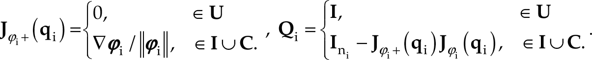
Visual Error Manifolds. Given that Q_i and J_φi+ (q_i) are orthogonal complements, and ${\dot{q}}_{\mathrm{i}}$ lies in the tangent plane at the contact point, a natural decomposition of ${\dot{q}}_{\mathrm{i}}$ that arises at the contact point can be defined as

$${\dot{q}}_{\mathrm{i}}\text{= }{Q}_{\mathrm{i}}{J}_{\mathrm{R}\mathrm{i}\mathrm{n}\mathrm{v}}{}_{{}_2}{\dot{x}}_{{\mathrm{s}}_{\mathrm{i}}}+J_{{\phi }_{\mathrm{i}+}}\left(q_{\mathrm{i}}\right){\dot{p}}_{\mathrm{i}}$$

(20)

where

$$Q_{\mathrm{i}}\text{ = }{I}_{{\mathrm{n}}_{\mathrm{i}}}-J_{{\phi }_{\mathrm{i}+}}\left(q_{\mathrm{i}}\right)J_{\phi \mathrm{i}}\left(q_{\mathrm{i}}\right)$$

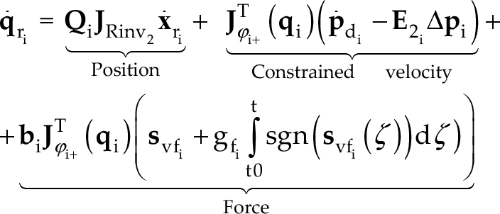
In order to assure the position and force tracking, the nominal visual position/force reference ${\dot{q}}_{\mathrm{r}\mathrm{i}}$ can be designed as

$$\begin{array}{l}{\dot{q}}_{{\mathrm{r}}_{\mathrm{i}}}\text{ = }\underset{\mathrm{P}\mathrm{o}\mathrm{s}\mathrm{i}\mathrm{t}\mathrm{i}\mathrm{o}\mathrm{n}}{\underbrace{Q_{\mathrm{i}}{J}_{\mathrm{R}\mathrm{i}\mathrm{n}{\mathrm{v}}_2}{\dot{x}}_{{\mathrm{r}}_{\mathrm{i}}}}}+\underset{\mathrm{C}\mathrm{o}\mathrm{n}\mathrm{s}\mathrm{t}\mathrm{r}\mathrm{a}\mathrm{i}\mathrm{n}\mathrm{e}\mathrm{d}\mathrm{v}\mathrm{e}\mathrm{l}\mathrm{o}\mathrm{c}\mathrm{i}\mathrm{t}\mathrm{y}}{\underbrace{J_{{\phi }_{\mathrm{i}+}}^{\mathrm{T}}\left(q_{\mathrm{i}}\right)\left({\dot{p}}_{{\mathrm{d}}_{\mathrm{i}}}-E_{2_{\mathrm{i}}}\Delta p_{\mathrm{i}}\right)}}+\\ +\underset{\mathrm{F}\mathrm{o}\mathrm{r}\mathrm{c}\mathrm{e}}{\underbrace{b_{\mathrm{i}}{J}_{{\phi }_{\mathrm{i}+}}^{\mathrm{T}}\left(q_{\mathrm{i}}\right)\left(s_{\mathrm{v}}{}_{{\mathrm{f}}_{\mathrm{i}}}+{\mathrm{g}}_{{\mathrm{f}}_{\mathrm{i}}}{\displaystyle \underset{\mathrm{t}0}{\overset{\mathrm{t}}{\int }}\mathrm{s}\mathrm{g}\mathrm{n}}\left(s_{\mathrm{v}{\mathrm{f}}_{\mathrm{i}}}\left(\zeta \right)\right)\mathrm{d}\zeta )\right)}}\end{array}$$

(21)

where ${\dot{x}}_{\mathrm{r}\mathrm{i}}$ stands for a visual nominal reference which parameterizes the system in terms of visual coordinates, E_2i is a positive definite diagonal matrix, $\nabla p_{\mathrm{i}}=p_{\mathrm{i}}-p_{{\mathrm{d}}_{\mathrm{i}}}=0,$ with $p_{{\mathrm{d}}_{\mathrm{i}}}$ the desired constraint position, and the subscript d_i denotes desired reference, b_i and ${\mathrm{g}}_{\mathrm{f}}{}_{{}_{\mathrm{i}}}$ are positive gain scalars, $s_{\mathrm{v}{\mathrm{f}}_{\mathrm{i}}}={\mathrm{s}}_{{\mathrm{f}}_{\mathrm{i}}}-{\mathrm{s}}_{\mathrm{d}{\mathrm{f}}_{\mathrm{i}}},{\mathrm{s}}_{{\mathrm{f}}_{\mathrm{i}}}=\Delta {\mathrm{f}}_{\mathrm{i}},\Delta {\mathrm{f}}_{\mathrm{i}}={\displaystyle {\int }_{{\mathrm{t}}_0}^{\mathrm{t}}\left({\lambda }_{\mathrm{i}}-{\lambda }_{{\mathrm{d}}_{\mathrm{i}}}\right)\left(\zeta \right)\mathrm{d}{\zeta }^2},{\lambda }_{{\mathrm{d}}_{\mathrm{i}}}$ the desired force, ${\mathrm{s}}_{\mathrm{d}{\mathrm{f}}_{\mathrm{i}}}={\mathrm{s}}_{{\mathrm{f}}_{\mathrm{i}}}\left({\mathrm{t}}_0\right){\mathrm{e}}^{-{\mathrm{k}}_{{\mathrm{f}}_{\mathrm{i}}}^{{\mathrm{t}}_0}},$ and the function sgn(y) is the discontinuous signum function of vector y.

Uncalibrated Joint Error Surface. Assuming that the parameters of the i-th manipulator are uncertainties and the parameters α, θ and b are not well known because the camera is not calibrated, this implies that the nominal reference defined previously in equation (21) cannot be used. Since we are interested in simultaneously controlling the visual position-force of the i-th manipulator, the noncalibrated nominal reference ${\dot{\stackrel{⌢}{\mathrm{q}}}}_{{\mathrm{r}}_{\mathrm{i}}}$ at the velocity level is

$$\begin{array}{l}{\dot{\stackrel{⌢}{\mathrm{q}}}}_{{\mathrm{r}}_{\mathrm{i}}}\text{ = }{Q}_{\mathrm{i}}{\stackrel{⌢}{J}}_{\mathrm{R}\mathrm{i}\mathrm{n}{\mathrm{v}}_2}{\dot{x}}_{{\mathrm{r}}_{\mathrm{i}}}+J_{{\phi }_{\mathrm{i}+}}\left(q_{\mathrm{i}}\right)\left({\dot{p}}_{{\mathrm{d}}_{\mathrm{i}}}-E_{2_{\mathrm{i}}}\Delta p_{\mathrm{i}}\right)+\\ +b_{\mathrm{i}}{J}_{{\phi }_{\mathrm{i}+}}^T\left(q_{\mathrm{i}}\right)\left(s_{\mathrm{v}}{}_{{\mathrm{f}}_{\mathrm{i}}}+{\mathrm{g}}_{{\mathrm{f}}_{\mathrm{i}}}{\displaystyle \underset{\mathrm{t}0}{\overset{\mathrm{t}}{\int }}\mathrm{s}\mathrm{g}\mathrm{n}}\left(s_{\mathrm{v}{\mathrm{f}}_{\mathrm{i}}}\right)\right)\end{array}$$

(22)

where ${\stackrel{⌢}{J}}_{\mathrm{R}\mathrm{i}\mathrm{n}{\mathrm{v}}_2}$ stands as an estimate of $J_{\mathrm{R}\mathrm{i}\mathrm{n}{\mathrm{v}}_2}$ so that the rank of ${\stackrel{⌢}{J}}_{\mathrm{R}\mathrm{i}\mathrm{n}{\mathrm{v}}_2}$ is n_i – m_i, for all t and for all q_i ∊ Ω. In addition, $E_{2\mathrm{i}},{\mathrm{g}}_{{\mathrm{f}}_{\mathrm{i}}}$ and $s_{\mathrm{v}}{}_{{\mathrm{f}}_{\mathrm{i}}},{\mathrm{b}}_{\mathrm{i}}$ are defined as in equation (21). Now, substituting (20) and (22) into equation (5), the uncertain visual error manifold becomes

$${\stackrel{⌢}{s}}_{\mathrm{i}}\text{ = }{Q}_{\mathrm{i}}\left(J_{\mathrm{R}\mathrm{i}\mathrm{n}{\mathrm{v}}_2}{\dot{x}}_{{\mathrm{s}}_{\mathrm{i}}}-{\stackrel{⌢}{J}}_{\mathrm{R}\mathrm{i}\mathrm{n}{\mathrm{v}}_2}{\dot{x}}_{{\mathrm{r}}_{\mathrm{i}}}\right)-J_{{\phi }_{\mathrm{i}+}}^{\mathrm{T}}\left(q_{\mathrm{i}}\right)\left(\Delta {\dot{p}}_{\mathrm{i}}+{\xi }_{2_{\mathrm{i}}}\Delta p_{\mathrm{i}}+b_{\mathrm{i}}{s}_{\mathrm{v}\mathrm{x}}{}_{{\mathrm{f}}_{\mathrm{i}}}\right)$$

(23)

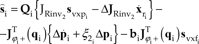
where $s_{\mathrm{v}\mathrm{x}}{}_{{\mathrm{f}}_{\mathrm{i}}}={\mathrm{s}}_{\mathrm{v}}{}_{{\mathrm{f}}_{\mathrm{i}}}+{\mathrm{g}}_{\mathrm{f}\mathrm{i}}{\displaystyle {\int }_{{\mathrm{t}}_0}^{\mathrm{t}}\mathrm{s}\mathrm{g}\mathrm{n}}\left({\mathrm{s}}_{\mathrm{v}}{}_{{\mathrm{f}}_{\mathrm{i}}}\right)$ is called the extended orthogonalized force manifold. In order to guarantee the tracking of the visual errors, a second order sliding mode is proposed through the nominal visual reference ${\dot{x}}_{{\mathrm{r}}_{\mathrm{i}}}$ given as

$${\dot{x}}_{{\mathrm{r}}_{\mathrm{i}}}={\dot{x}}_{\mathrm{s}{\mathrm{d}}_{\mathrm{i}}}-A_{\mathrm{i}}\Delta x_{\mathrm{s}}{}_{{}_{\mathrm{i}}}+s_{\mathrm{d}{\mathrm{p}}_{\mathrm{i}}}-G_{{\mathrm{p}}_{\mathrm{i}}}{\displaystyle \underset{\mathrm{t}0}{\overset{\mathrm{t}}{\int }}\mathrm{s}\mathrm{g}\mathrm{n}\left(s_{{\mathrm{x}}_{\mathrm{i}}}\right)}$$

(24)

where $A_{\mathrm{i}},G_{{\mathrm{p}}_{\mathrm{i}}},$ are positive-definite diagonal matrices, $\Delta x_{\mathrm{s}}{}_{{}_{\mathrm{i}}}=x_{\mathrm{s}}{}_{{}_{\mathrm{i}}}-x_{\mathrm{s}{\mathrm{d}}_{\mathrm{i}}},$ and $s_{\mathrm{d}\mathrm{p}}{}_{{}_{\mathrm{i}}}=s_{{\mathrm{x}}_{\mathrm{i}}}\left({\mathrm{t}}_0\right)\mathrm{e}\mathrm{x}{\mathrm{p}}^{-{\mathrm{k}}_{\mathrm{p}\mathrm{i}}}{}^{(\mathrm{t}-\mathrm{t}0)}$ with $s_{{\mathrm{x}}_{\mathrm{i}}}=\Delta x_{\mathrm{s}}{}_{{}_{\mathrm{i}}}+A_{\mathrm{i}}\Delta x_{{\mathrm{s}}_{\mathrm{i}}}.$ Given that the sliding mode condition is satisfied for $s_{{\mathrm{x}}_{\mathrm{i}}}$ , and not for ${\stackrel{⌢}{s}}_{\mathrm{i}},$ we have that the switching over the Cartesian manifold will be invariant to parametric uncertainties thanks to ${\dot{x}}_{{\mathrm{r}}_{\mathrm{i}}}.$

Open Loop Error Dynamics. The parametrization of the i-th robot manipulator (see equation (3)), requires the derivative of equation (22), which is discontinuous. Given that we will use neural networks to handle the entire system, we will simplify the equation (3) in order to avoid discontinuous signals. One way of doing this is to decompose ${\ddot{q}}_{{\mathrm{r}}_{\mathrm{i}}}$ into continuous and discontinuous terms as follows

$${\ddot{\stackrel{⌢}{\mathrm{q}}}}_{{\mathrm{r}}_{\mathrm{i}}}\text{ = }{\ddot{\stackrel{⌢}{\mathrm{q}}}}_{\mathrm{c}\mathrm{o}\mathrm{n}{\mathrm{t}}_{\mathrm{i}}}+{\ddot{\stackrel{⌢}{\mathrm{q}}}}_{\mathrm{d}\mathrm{i}\mathrm{s}{\mathrm{c}}_{\mathrm{i}}}$$

(25)

with

$$\begin{array}{l}{\ddot{\stackrel{⌢}{q}}}_{\mathrm{con}{\mathrm{t}}_{\mathrm{i}}}={\dot{Q}}_{\text{i}}{\stackrel{⌢}{J}}_{{\text{Rinv}}_{\text{i}2}}{\dot{x}}_{{\text{r}}_{\mathrm{i}}}+Q_{\text{i}}{\dot{\stackrel{⌢}{J}}}_{{\text{Rinv}}_{\text{i}2}}{\dot{x}}_{{\text{r}}_{\mathrm{i}}}+Q_{\text{i}}{J}_{{\text{Rinv}}_{\text{i}2}}\left(x_{{\text{sd}}_{\text{i}}}-A_{\text{i}}\Delta {\dot{x}}_{{\text{s}}_{\mathrm{i}}}+{\dot{s}}_{{\text{sp}}_{\text{i}}}-G_{{\text{p}}_{\mathrm{i}}}\tanh \left({\lambda }_{{\text{p}}_{\mathrm{i}}}{s}_{{\text{x}}_{\mathrm{i}}}\right)\right)\hfill \\ +b_{\text{i}}{\dot{J}}_{{\phi }_{\text{i}}}^{\text{T}}\left(q_{\text{i}}\right)s_{{\text{vxf}}_{\text{i}}}+b_{\text{i}}{J}_{{\phi }_{\text{i}}}^{\text{T}}\left(q_{\text{i}}\right)\left(\Delta {\text{f}}_{\mathrm{i}}-{\dot{s}}_{{\text{df}}_{\text{i}}}+{\text{g}}_{{\text{f}}_{\mathrm{i}}}\tanh \left({\lambda }_{{\text{f}}_{\mathrm{i}}}{s}_{{\text{vf}}_{\text{i}}}\right)\right)\hfill \\ {\ddot{\stackrel{⌢}{q}}}_{\mathrm{dis}{\mathrm{c}}_{\mathrm{i}}}=Q_{\text{i}}{\stackrel{⌢}{J}}_{{\text{Rinv}}_{\text{i}2}}{z}_{{\text{p}}_{\mathrm{i}}}-b_{\text{i}}{J}_{{\phi }_{\text{i}}}^{\text{T}}\left(q_{\text{i}}\right)z_{{\text{f}}_{\mathrm{i}}}\hfill \end{array}$$

with $z_{\mathrm{p}\mathrm{i}}=\tanh \left({\lambda }_{{\mathrm{p}}_{\mathrm{i}}}{s}_{{\mathrm{x}}_{\mathrm{i}}}\right)-\mathrm{s}\mathrm{g}\mathrm{n}\left(s_{{\mathrm{x}}_{\mathrm{i}}}\right)$ , $z_{{\mathrm{f}}_{\mathrm{i}}}=\tanh \left({\lambda }_{{\mathrm{f}}_{\mathrm{i}}}{s}_{\mathrm{v}{\mathrm{f}}_{\mathrm{i}}}\right)-\mathrm{s}\mathrm{g}\mathrm{n}\left(s_{\mathrm{v}{\mathrm{f}}_{\mathrm{i}}}\right),$ and ${\lambda }_{{\mathrm{p}}_{\mathrm{i}}},{\lambda }_{{\mathrm{f}}_{\mathrm{i}}}∊{\Re }^{\mathrm{n}\times \mathrm{n}}>0.$ . The continuous function tanh(*) is used as approximation of discontinuous function sgn(*), such that tanh(0) = 0 and $\tanh \left({\lambda }_{{\mathrm{p}}_{\mathrm{i}}}{s}_{{\mathrm{x}}_{\mathrm{i}}}\right)\to \mathrm{s}\mathrm{g}\mathrm{n}\left(s_{{\mathrm{x}}_{\mathrm{i}}}\right),\tanh \left({\lambda }_{{\mathrm{f}}_{\mathrm{i}}}{s}_{\mathrm{v}{\mathrm{f}}_{\mathrm{i}}}\right)\to \mathrm{s}\mathrm{g}\mathrm{n}\left(s_{\mathrm{v}{\mathrm{f}}_{\mathrm{i}}}\right)$ when ${\lambda }_{\mathrm{i}}\to \infty .$ . Notice that $z_{{\mathrm{p}}_{\mathrm{i}}},z_{{\mathrm{f}}_{\mathrm{i}}}$ have the following properties: ${\mathrm{z}}_{\mathrm{x}}\ge -1,{\mathrm{z}}_{\mathrm{x}}\le +1.$ Finally, the parametrization of (3) using the equations (22) and (25) gives rise to

$$H_{\mathrm{i}}\left(q_{\mathrm{i}}\right){\ddot{\stackrel{⌢}{\mathrm{q}}}}_{{\mathrm{r}}_{\mathrm{i}}}+C_{\mathrm{i}}\left(q_{\mathrm{i}},{\dot{q}}_{\mathrm{i}}\right){\dot{\stackrel{⌢}{\mathrm{q}}}}_{{\mathrm{r}}_{\mathrm{i}}}+g_{\mathrm{i}}\left(q_{\mathrm{i}}\right)=Y_{\mathrm{c}\mathrm{o}\mathrm{n}{\mathrm{t}}_{\mathrm{i}}}{\stackrel{⌢}{m}}_{\mathrm{i}}+u_{{\mathrm{d}}_{\mathrm{i}}}$$

(26)

where $Y_{\mathrm{c}\mathrm{o}\mathrm{n}{\mathrm{t}}_{\mathrm{i}}}=Y_{{\mathrm{b}}_{\mathrm{i}}}\left(q_{\mathrm{i}},{\dot{q}}_{\mathrm{i}},{\ddot{\stackrel{⌢}{\mathrm{q}}}}_{{\mathrm{r}}_{\mathrm{i}}},{\ddot{\stackrel{⌢}{\mathrm{q}}}}_{\mathrm{c}\mathrm{o}\mathrm{n}{\mathrm{t}}_{\mathrm{i}}}\right)$ is continuous due to $\left({\ddot{\stackrel{⌢}{\mathrm{q}}}}_{{\mathrm{r}}_{\mathrm{i}}},{\ddot{\stackrel{⌢}{\mathrm{q}}}}_{\mathrm{c}\mathrm{o}\mathrm{n}{\mathrm{t}}_{\mathrm{i}}}\right)∊{\mathrm{C}}^1$ and $u_{{\mathrm{d}}_{\mathrm{i}}}=H_{\mathrm{i}}\left({\dot{q}}_{\mathrm{i}}\right){\ddot{q}}_{\mathrm{d}\mathrm{i}\mathrm{s}{\mathrm{c}}_{\mathrm{i}}}$ is considered as an endogenous bounded disturbance subject to matching conditions. It is important to notice that $u_{{\mathrm{d}}_{\mathrm{i}}}$ cannot be compensated by the neural network, because it is discontinuous. However, $u_{{\mathrm{d}}_{\mathrm{i}}}$ is bounded due to $z_{{\mathrm{p}}_{\mathrm{i}}}$ and $z_{{\mathrm{f}}_{\mathrm{i}}}$ being bounded. Adding and subtracting equation (26) into equation (1), the open loop error equation arises as

$$H_{\mathrm{i}}\left(q_{\mathrm{i}}\right){\dot{\stackrel{⌢}{\mathrm{s}}}}_{\mathrm{i}}+C_{\mathrm{i}}\left(q_{\mathrm{i}},{\dot{q}}_{\mathrm{i}}\right){\stackrel{⌢}{s}}_{\mathrm{i}}=u_{\mathrm{i}}-Y_{\mathrm{c}\mathrm{o}\mathrm{n}{\mathrm{t}}_{\mathrm{i}}}{\stackrel{⌢}{m}}_{\mathrm{i}}+J_{{\phi }_{\mathrm{i}+}}^{\mathrm{T}}\left(q_{\mathrm{i}}\right){\lambda }_{\mathrm{i}}+u_{{\mathrm{d}}_{\mathrm{i}}}$$

(27)

It remains now to design the controller u _i that satisfies the problem raised. Our controller will compensate $Y_{\mathrm{c}\mathrm{o}\mathrm{n}{\mathrm{t}}_{\mathrm{i}}}{\stackrel{⌢}{m}}_{\mathrm{i}}$ with a low dimensional neural network, while the approximation error of the i-th neural network and $z_{{\mathrm{p}}_{\mathrm{i}}}$ , $z_{{\mathrm{f}}_{\mathrm{i}}}$ in $u_{{\mathrm{d}}_{\mathrm{i}}}$ will be compensated with an orthogonalized second order sliding mode inner loop. At this stage, before designing u_i, we discuss the design of the neural network architecture as an associator to approximated $Y_{\mathrm{c}\mathrm{o}\mathrm{n}{\mathrm{t}}_{\mathrm{i}}}{\stackrel{⌢}{m}}_{\mathrm{i}}$ .

4. Uncertain neuro-visual based controller

4.1 Neural Network Architecture

A tree network structure that satisfies the Stone-Weierstrass theorem [2] is used to approximate continuous regressor $Y_{\mathrm{c}\mathrm{o}\mathrm{n}{\mathrm{t}}_{\mathrm{i}}},$ i.e., many neurons on one layer feed a single neuron on the next layer. The input-output relationship for this generic architecture is given as ${\mathrm{y}}_{\mathrm{i}}=\phi \left({\displaystyle {\sum }_{\mathrm{k}=1}^{\mathrm{m}}{\mathrm{x}}_{\mathrm{k}}{\mathrm{w}}_{\mathrm{k}}}\right),$ where x_k is the k-th input to the neural network, w_k is the k-th weight, and ϕ the activation function. Notice that tree structure could have one or more hidden layers, where the linear activation function is used as the last stage of a multilayer neural network. Considering the property that neural networks can approximate any smooth function f(x), where φ belongs to a compact set s of Rⁿ [3], [11], we can use a sufficiently large neural network to approximate some function f(x) such that

$$\underset{{\tilde{\mathrm{w}}}_{\mathrm{i}}}{\min }\left|f\left(x\right)-\stackrel{⌢}{f}\left(x,\tilde{w}\right)\right|$$

with $\stackrel{⌢}{\mathrm{f}}\left(x,\tilde{w}\right)\equiv \phi \left(x·\tilde{w}\right),$ and $\Vert \tilde{w}\Vert \le {\mathrm{w}}_{\mathrm{m}\mathrm{a}\mathrm{x}},$ is minimized.

Given that the regressor $Y_{\mathrm{c}\mathrm{o}\mathrm{n}{\mathrm{t}}_{\mathrm{i}}}$ is continuous, it will be approximated by an ADAptive LINear Element (ADALINE) [20], which consists of a single neuron of the McCulloch-Pitts type. Using a matrix representation, the approximator will be designed such that

$$\underset{{\tilde{\mathrm{w}}}_{\mathrm{i}}}{\min }\Vert Y_{\mathrm{c}\mathrm{o}\mathrm{n}{\mathrm{t}}_{\mathrm{i}}}{\stackrel{⌢}{m}}_{\mathrm{i}}-{\stackrel{⌢}{f}}_{\mathrm{i}}\left(X_{\mathrm{i}},{\tilde{w}}_{\mathrm{i}}\right)\Vert$$

with ${\stackrel{⌢}{f}}_{\mathrm{i}}\left(X_{\mathrm{i}},{\tilde{w}}_{\mathrm{i}}\right)\equiv X_{\mathrm{i}}^{\mathrm{T}}{\tilde{w}}_{\mathrm{i}},X_{\mathrm{i}}^{\mathrm{T}}=\left[q_{\mathrm{i}},{\dot{q}}_{\mathrm{i}},{\ddot{\stackrel{⌢}{\mathrm{q}}}}_{{\mathrm{r}}_{\mathrm{i}}},{\ddot{\stackrel{⌢}{\mathrm{q}}}}_{\mathrm{c}\mathrm{o}\mathrm{n}{\mathrm{t}}_{\mathrm{i}}}\right]∊{\Re }^{{\mathrm{n}}_{\mathrm{i}}\times {\mathrm{p}}_{\mathrm{i}}},{\tilde{w}}_{\mathrm{i}}∊{\Re }^{{\mathrm{p}}_{\mathrm{i}}},$ and $\Vert {\tilde{w}}_{\mathrm{i}}\Vert \le {\mathrm{w}}_{\mathrm{m}\mathrm{a}\mathrm{x}},$ is minimized. Thus, the low dimensional neural network is used to approximate the unknown function $f(x)=Y_{\mathrm{c}\mathrm{o}\mathrm{n}{\mathrm{t}}_{\mathrm{i}}}{\stackrel{⌢}{m}}_{\mathrm{i}}$ by

$$\stackrel{⌢}{f}\left(x\right)=X_{\mathrm{i}}^{\mathrm{T}}{\tilde{w}}_{\mathrm{i}}+e_{\mathrm{i}}\left(X_{\mathrm{i}}\right)$$

(28)

where $X_{\mathrm{T}}^{\mathrm{i}}$ are the inputs to the neural network, ${\tilde{w}}_{\mathrm{i}}$ are the estimated neural network weights for the i-th manipulator and $\Vert {\mathrm{e}}_{\mathrm{i}}\left(X_{\mathrm{i}}\right)\Vert \le {∊}_{\mathrm{N}}$ is a functional reconstruction error with ∊_N > 0.

Given that the size of the neural network is defined by taking into account only the regressor elements, its approximation capacity is severely limited. However, instead of increasing its number of neurons in order to reduce the residual error, the error will be eliminated by means of a training procedure based on an orthogonalized second order sliding mode.

4.2 Neural-Visual Controller Design

Substituting equation (28) into equation (27), we have

$$H_{\mathrm{i}}\left(q_{\mathrm{i}}\right){\dot{\stackrel{⌢}{\mathrm{s}}}}_{\mathrm{i}}+C_{\mathrm{i}}\left(q_{\mathrm{i}},{\dot{q}}_{\mathrm{i}}\right){\stackrel{⌢}{s}}_{\mathrm{i}}=u_{\mathrm{i}}-X_{\mathrm{i}}{\stackrel{⌢}{w}}_{\mathrm{i}}+J_{{\phi }_{\mathrm{i}}+}^{\mathrm{T}}\left(q_{\mathrm{i}}\right){\lambda }_{\mathrm{i}}+{\overline{u}}_{\mathrm{d}}$$

(29)

where ${\overline{u}}_{\mathrm{d}}=u_{{\mathrm{d}}_{\mathrm{i}}}-e_{\mathrm{i}}(X_{\mathrm{i}}).$

Now we are ready to present the main result.

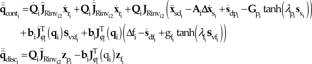
Theorem 4.1. Assume that all initial conditions and desired trajectories of the i-th manipulator belong to Ω. Consider the dynamical model of the i-th manipulator in the closed-loop with the control law and neuro-adaptive law defined as

$$\begin{array}{l}{u}_{\mathrm{i}}=-K_{{\mathrm{d}}_{\mathrm{i}}}{\stackrel{⌢}{s}}_{\mathrm{i}}+x_{\mathrm{i}}^{\mathrm{T}}{\stackrel{⌢}{w}}_{\mathrm{i}}+J_{{\phi }_{\mathrm{i}}+}^{\mathrm{T}}\left(q_{\mathrm{i}}\right)\left(-{\lambda }_{{\mathrm{d}}_{\mathrm{i}}}+{\eta }_{\mathrm{i}}\Delta {\mathrm{f}}_{\mathrm{i}}\right)\\ +{\gamma }_{{\mathrm{F}}_{\mathrm{i}}}{J}_{{\phi }_{\mathrm{i}}}^{\mathrm{T}}\left(q_{\mathrm{i}}\right)\left(\tanh \left({\mu }_{\mathrm{i}}{s}_{\mathrm{v}{\mathrm{f}}_{\mathrm{i}}}\right)+{\eta }_{\mathrm{i}}{\displaystyle {\int }_{{\mathrm{t}}_0}^{\mathrm{t}}\mathrm{s}\mathrm{g}\mathrm{n}\left(s_{\mathrm{v}{\mathrm{f}}_{\mathrm{i}}}\right)}\right)\end{array}$$

(30)

$${\dot{\stackrel{⌢}{\mathrm{w}}}}_{\mathrm{i}}=-{\Gamma }_{\mathrm{i}}{X}_{\mathrm{i}}{\stackrel{⌢}{s}}_{\mathrm{i}}$$

(31)

where $K_{{\mathrm{d}}_{\mathrm{i}}}∊{\Re }^{{\mathrm{n}}_{\mathrm{i}}\times {\mathrm{n}}_{\mathrm{i}}},{\stackrel{⌢}{w}}_{\mathrm{i}}∊{\Re }^{{\mathrm{p}}_{\mathrm{i}}},{\Gamma }_{\mathrm{i}}∊{\Re }^{{\mathrm{p}}_{\mathrm{i}}\times {\mathrm{p}}_{\mathrm{i}}}$ and ${\lambda }_{{\mathrm{d}}_{\mathrm{i}}}$ is the i-th desired contact force. Then, for small initial conditions and large enough feedback gain matrix $K_{{\mathrm{d}}_{\mathrm{i}}},$ there is exponential convergence of the visual position error and force tracking error despite the existence of parametric uncertainties in ${\stackrel{⌢}{J}}_{\mathrm{R}\mathrm{i}\mathrm{n}{\mathrm{v}}_{\mathrm{i}2}}.$ .

Substituting equation (30) into equation (29), the closed-loop equation becomes

$$\begin{array}{l}{H}_{\mathrm{i}}\left(q_{\mathrm{i}}\right){\dot{\stackrel{⌢}{\mathrm{s}}}}_{\mathrm{i}}+C_{\mathrm{i}}\left(q_{\mathrm{i}},{\dot{q}}_{\mathrm{i}}\right){\stackrel{⌢}{s}}_{\mathrm{i}}=\\ =-K_{{\mathrm{d}}_{\mathrm{i}}}{\stackrel{⌢}{s}}_{\mathrm{i}}+x_{\mathrm{i}}^{\mathrm{T}}\Delta w_{\mathrm{i}}+J_{{\phi }_{\mathrm{i}}+}^{\mathrm{T}}\left(q_{\mathrm{i}}\right)\left({\dot{s}}_{\mathrm{v}{\mathrm{f}}_{\mathrm{i}}}+{\eta }_{\mathrm{i}}{s}_{\mathrm{v}{\mathrm{f}}_{\mathrm{i}}}\right)+{\overline{\mathrm{u}}}_{\mathrm{d}}\end{array}$$

(32)

where $\Delta w_{\mathrm{i}}={\stackrel{⌢}{w}}_{\mathrm{i}}-{\tilde{w}}_{\mathrm{i}}.$

Proof: The proof is divided in three parts:

Part I. [Boundedness of Closed-loop Trajectories] Consider the time derivative of the following Lyapunov candidate function

$$\mathrm{V}=\frac{1}{2}{\displaystyle \sum _{\mathrm{i}=1}^{\mathrm{l}}\left({\stackrel{⌢}{s}}_{\mathrm{i}}^{\mathrm{T}}{H}_{\mathrm{i}}\left(q_{\mathrm{i}}\right){\stackrel{⌢}{s}}_{\mathrm{i}}+b_{\mathrm{i}}{s}_{\mathrm{v}{\mathrm{f}}_{\mathrm{i}}}^{\mathrm{T}}{s}_{\mathrm{v}{\mathrm{f}}_{\mathrm{i}}}^{}+\Delta w_{\mathrm{i}}^{\mathrm{T}}{\Gamma }_{\mathrm{i}}^{-1}\Delta w_{\mathrm{i}}\right)}$$

(33)

along the solutions of (32), then it yields

$$\dot{\mathrm{V}}\le {\displaystyle \sum _{\mathrm{i}=1}^{\mathrm{l}}\left(-{\stackrel{⌢}{s}}_{\mathrm{i}}^{\mathrm{T}}{K}_{{\mathrm{d}}_{\mathrm{i}}}{\stackrel{⌢}{s}}_{\mathrm{i}}-{\eta }_{\mathrm{i}}{b}_{\mathrm{i}}{s}_{\mathrm{v}{\mathrm{f}}_{{}_{\mathrm{i}}}}^{\mathrm{T}}{s}_{\mathrm{v}{\mathrm{f}}_{{}_{\mathrm{i}}}}^{}+\Vert {\stackrel{⌢}{s}}_{{\mathrm{r}}_{\mathrm{i}}}\Vert {\overline{u}}_{\mathrm{d}}\right)}$$

(34)

where ${\stackrel{⌢}{s}}_{\mathrm{i}}^{\mathrm{T}}{\overline{u}}_{\mathrm{d}}$ is radially unbounded only when ${\stackrel{⌢}{s}}_{\mathrm{i}}\to \infty$ and for bounded signals ${\stackrel{⌢}{s}}_{\mathrm{i}}^{\mathrm{T}}{\overline{u}}_{\mathrm{d}}$ is zero only at ${\stackrel{⌢}{s}}_{\mathrm{i}}^{\mathrm{T}}=0.$ For the small initial errors belonging to a neighbourhood ∊₁ and ∊₂ centred in the equilibriums ${\stackrel{⌢}{s}}_{\mathrm{i}}=0$ and ${\stackrel{⌢}{s}}_{\mathrm{v}{\mathrm{f}}_{\mathrm{i}}}=0,$ there exists a large enough feedback gain matrix $K_{{\mathrm{d}}_{\mathrm{i}}}$ such that each of the components of ${\stackrel{⌢}{s}}_{\mathrm{i}}$ converges to ∊₁ > 0 as t → ∞, and ${\stackrel{⌢}{s}}_{\mathrm{v}{\mathrm{f}}_{\mathrm{i}}}$ also converge to ∊₂ > 0 when t → ∞. This result stands for local stability of ${\stackrel{⌢}{s}}_{\mathrm{i}}$ provided that the state is near the desired trajectories for any initial conditions. The boundedness in the L∞ sense leads to the existence of the constant ∊₃ > 0 such that

$$\Vert {\stackrel{⌢}{s}}_{\mathrm{i}}\Vert \le {∊}_3$$

Since desired trajectories are C² and feedback gains are bounded, we have that $\left({\dot{q}}_{\mathrm{r}\mathrm{i}},{\ddot{q}}_{\mathrm{c}\mathrm{o}\mathrm{n}{\mathrm{t}}_{\mathrm{i}}}\right)∊\mathrm{L}\infty ,$ which implies that $Y_{\mathrm{c}\mathrm{o}\mathrm{n}{\mathrm{t}}_{\mathrm{i}}}∊\mathrm{L}\infty ,X_{\mathrm{i}}∊\mathrm{L}\infty$ and ${\dot{\stackrel{⌢}{\mathrm{w}}}}_{\mathrm{i}}∊\mathrm{L}\infty .$ Then, the output of the neural network is also bounded. According the previous arguments and the boundedness of the i-th robot dynamics, its Coriolis matrix and gravitational term, and given that inertia matrix is positive-definite and upper bounded, the right hand side of equation (32) is bounded, such that ${\dot{\stackrel{⌢}{\mathrm{s}}}}_{\mathrm{i}}∊\mathrm{L}\infty .$ Then, there exists a bounded scalar ∊₄ > 0 such that

$$\Vert {\dot{\stackrel{⌢}{\mathrm{s}}}}_{\mathrm{i}}\Vert \le {∊}_4$$

So far, we can conclude the boundedness of all closed-loop error signals. To prove convergence of tracking errors, the sliding modes condition must be verified in the force subspace $J_{{\phi }_{\mathrm{i}+}}^{\mathrm{T}}$ and in the position subspace Q_i.

Part II.a [Sliding modes for the velocity subspace]. Adding and subtracting $Q_{\mathrm{i}}{\mathrm{J}}_{\mathrm{R}\mathrm{i}\mathrm{n}{\mathrm{v}}_2}{\dot{x}}_{{\mathrm{r}}_{\mathrm{i}}}$ to (23), we obtain

$$\begin{array}{l}{\stackrel{⌢}{s}}_{\mathrm{i}}=Q_{\mathrm{i}}\left\{{\mathrm{J}}_{\mathrm{R}\mathrm{i}\mathrm{n}{\mathrm{v}}_2}{s}_{\mathrm{v}\mathrm{x}{\mathrm{p}}_{\mathrm{i}}}-\Delta J_{\mathrm{R}\mathrm{i}\mathrm{n}{\mathrm{v}}_2}{\dot{x}}_{{\mathrm{r}}_{\mathrm{i}}}\right\}-\\ -J_{{\phi }_{\mathrm{i}}+}^{\mathrm{T}}\left(q_{\mathrm{i}}\right)\left\{\Delta {\dot{p}}_{\mathrm{i}}+{\xi }_{2_{\mathrm{i}}}\Delta p_{\mathrm{i}}\right\}-b_{\mathrm{i}}{J}_{{\phi }_{\mathrm{i}}+}^{\mathrm{T}}\left(q_{\mathrm{i}}\right)s_{\mathrm{v}\mathrm{x}{\mathrm{f}}_{\mathrm{i}}}\end{array}$$

(35)

where $s_{\mathrm{v}\mathrm{x}{\mathrm{p}}_{\mathrm{i}}}={\mathrm{s}}_{\mathrm{v}{\mathrm{p}}_{\mathrm{i}}}+{\gamma }_{{\mathrm{p}}_{\mathrm{i}}}{\displaystyle {\int }_{{\mathrm{t}}_0}^{\mathrm{t}}\mathrm{s}\mathrm{g}\mathrm{n}}\left({\mathrm{s}}_{\mathrm{v}{\mathrm{p}}_{\mathrm{i}}}\right)$ is called extended orthogonalized position manifold and $\Delta J_{\mathrm{R}\mathrm{i}\mathrm{n}{\mathrm{v}}_2}={\stackrel{⌢}{J}}_{\mathrm{R}\mathrm{i}\mathrm{n}{\mathrm{v}}_2}-J_{\mathrm{R}\mathrm{i}\mathrm{n}{\mathrm{v}}_2}<\sigma ,$ for σ > 0 under the assumption that $J_{\mathrm{R}\mathrm{i}\mathrm{n}{\mathrm{v}}_2}$ is not degenerated in Ω, and ${\stackrel{⌢}{J}}_{\mathrm{R}\mathrm{i}\mathrm{n}{\mathrm{v}}_2}$ is composed by trigonometric functions. Now, since ${\stackrel{⌢}{s}}_{\mathrm{i}}∊\mathrm{L}\infty ,\phi \left(q\right)$ is smooth and lies in the reachable robot space Ω, and $J_{\mathrm{R}\mathrm{i}\mathrm{n}{\mathrm{v}}_2}$ and Q_i are bounded, we have that $\frac{\mathrm{d}}{\mathrm{d}\mathrm{t}}{Q}_{\mathrm{i}}{J}_{{\text{Rinv}}_2}{s}_{{\mathrm{v}\mathrm{x}\mathrm{p}}_{\mathrm{i}}}$ and $\frac{\mathrm{d}}{\mathrm{d}\mathrm{t}}$ $J_{{\phi }_{\mathrm{i}}+}^{\mathrm{T}}{s}_{\mathrm{v}\mathrm{x}{\mathrm{f}}_{\mathrm{i}}}$ are bounded (this is possible because ${\dot{J}}_{{\phi }_{\mathrm{i}}}^{\mathrm{T}}$ and Q_i are bounded). Then, there exist bounded constants ∊₅ > 0 and ∊₆ > 0 such that

$$\left|{\dot{s}}_{\mathrm{v}\mathrm{x}{\mathrm{p}}_{\mathrm{i}}}\right|\text{< }{∊}_5,\left|{\dot{s}}_{\mathrm{v}\mathrm{x}{\mathrm{f}}_{\mathrm{i}}}\right|\text{< }{∊}_6$$

Multiplying (35) by $Q_{\mathrm{T}}^{\mathrm{i}}$ and rearranging terms we obtain

$$\begin{array}{l}{Q}_{\mathrm{i}}^{\mathrm{T}}{\stackrel{⌢}{s}}_{\mathrm{i}}=Q_{\mathrm{i}}^{\mathrm{T}}{Q}_{\mathrm{i}}\left\{J_{\mathrm{R}\mathrm{i}\mathrm{n}{\mathrm{v}}_2}{s}_{\mathrm{v}\mathrm{x}{\mathrm{p}}_{\mathrm{i}}}-\Delta J_{\mathrm{R}\mathrm{i}\mathrm{n}{\mathrm{v}}_2}{\dot{x}}_{{\mathrm{r}}_{\mathrm{i}}}\right\}-\\ -\underset{=0}{\underbrace{Q_{\mathrm{i}}^{\mathrm{T}}{J}_{{\phi }_{\mathrm{i}}+}^{\mathrm{T}}\left(q_{\mathrm{i}}\right)\left\{\Delta {\dot{p}}_{\mathrm{i}}+{\xi }_{2_{\mathrm{i}}}\Delta p_{\mathrm{i}}\right\}}}-\underset{=0}{\underbrace{{\mathrm{b}}_{\mathrm{i}}{Q}_{\mathrm{i}}^{\mathrm{T}}{\mathrm{J}}_{{\phi }_{\mathrm{i}}+}^{\mathrm{T}}\left(q_{\mathrm{i}}\right)s_{\mathrm{v}\mathrm{x}{\mathrm{f}}_{\mathrm{i}}}}}\end{array}$$

(36)

and

$$\begin{array}{l}{J}_{\mathrm{R}\mathrm{i}\mathrm{n}{\mathrm{v}}_2}{s}_{\mathrm{v}\mathrm{x}{\mathrm{p}}_{\mathrm{i}}}=Q_{\mathrm{i}}^{\Delta }{\stackrel{⌢}{s}}_{\mathrm{i}}+\Delta J_{\mathrm{R}\mathrm{i}\mathrm{n}{\mathrm{v}}_2}{\dot{x}}_{{\mathrm{r}}_{\mathrm{i}}}\\ {\overline{s}}_{\mathrm{v}\mathrm{x}{\mathrm{p}}_{\mathrm{i}}}=Q_{\mathrm{i}}^{\Delta }{\stackrel{⌢}{s}}_{\mathrm{i}}+\Delta J_{\mathrm{R}\mathrm{i}\mathrm{n}{\mathrm{v}}_2}{\dot{x}}_{{\mathrm{r}}_{\mathrm{i}}}\end{array}$$

(37)

where $Q_{\mathrm{i}}^{\Delta }={\left(Q_{\mathrm{i}}^{\mathrm{T}}{Q}_{\mathrm{i}}\right)}^{-1}{Q}_{\mathrm{i}}^{\mathrm{T}}$ and ${\overline{s}}_{\mathrm{v}\mathrm{p}{\mathrm{x}}_{\mathrm{i}}}$ is the local projection of $s_{\mathrm{v}\mathrm{p}{\mathrm{x}}_{\mathrm{i}}}$ onto $\mathrm{i}\mathrm{m}\left({\overline{J}}_2\right).$ Given that there are n_i – m_i independent coordinates, and m_i dependent coordinates can be expressed as a function of independent coordinates, then the holonomic constraint is well posed. That is, once a solution (given by a initial condition) is chosen, this solution cannot jump to another solution of $J_{\mathrm{R}\mathrm{i}\mathrm{n}{\mathrm{v}}_1}$ since we have ruled out crossing singularities, so it stays always in the domain of this solution. Then this local domain in fact becomes the global domain of this solution. So, it is reasonable to assume a bijection in this domain, between ${\overline{s}}_{\mathrm{v}\mathrm{p}{\mathrm{x}}_{\mathrm{i}}}$ and $s_{\mathrm{v}\mathrm{p}{\mathrm{x}}_{\mathrm{i}}}$ . Hence, without loss of generality we can analyse either ${\overline{s}}_{\mathrm{v}\mathrm{p}{\mathrm{x}}_{\mathrm{i}}}$ or $s_{\mathrm{v}\mathrm{p}{\mathrm{x}}_{\mathrm{i}}}$ . Taking into account the definition of $s_{\mathrm{v}\mathrm{p}{\mathrm{x}}_{\mathrm{i}}}$ , (37) becomes

$$s_{\mathrm{v}{\mathrm{p}}_{\mathrm{i}}}=-{\gamma }_{\mathrm{p}\mathrm{i}}{\displaystyle {\int }_{{\mathrm{t}}_0}^{\mathrm{t}}\mathrm{s}\mathrm{g}\mathrm{n}\left(s_{\mathrm{v}{\mathrm{p}}_{\mathrm{i}}}\right)}+\underset{\mathrm{a}}{\underbrace{Q_{\mathrm{i}}^{\Delta }{\stackrel{⌢}{s}}_{\mathrm{i}}+\Delta J_{\mathrm{R}\mathrm{i}\mathrm{n}{\mathrm{v}}_2}{\dot{x}}_{{\mathrm{r}}_{\mathrm{i}}}}}$$

(38)

Multiplying the time derivative of the equation (38) by $s_{\mathrm{v}{\mathrm{p}}_{\mathrm{i}}}^{\mathrm{T}}$ , we obtain that

$$\begin{array}{l}{s}_{\mathrm{v}{\mathrm{p}}_{\mathrm{i}}}^{\mathrm{T}}{\dot{s}}_{\mathrm{v}{\mathrm{p}}_{\mathrm{i}}}=s_{\mathrm{v}{\mathrm{p}}_{\mathrm{i}}}^{\mathrm{T}}\left(-{\gamma }_{\mathrm{p}\mathrm{i}}\mathrm{s}\mathrm{g}\mathrm{n}\left(s_{\mathrm{v}{\mathrm{p}}_{\mathrm{i}}}\right)+\frac{\mathrm{d}}{\mathrm{d}\mathrm{t}}\mathrm{a}\right)\\ \le -{\gamma }_{\mathrm{p}\mathrm{i}}\left|s_{\mathrm{v}{\mathrm{p}}_{\mathrm{i}}}\right|+\left|s_{\mathrm{v}{\mathrm{p}}_{\mathrm{i}}}\right|\left|\frac{\mathrm{d}}{\mathrm{d}\mathrm{t}}\mathrm{a}\right|\\ \le -{\gamma }_{\mathrm{p}\mathrm{i}}\left|s_{\mathrm{v}{\mathrm{p}}_{\mathrm{i}}}\right|+{∊}_7\left|s_{\mathrm{v}\mathrm{p}}\right|\\ \le -\left({\gamma }_{\mathrm{p}}-{∊}_7\right)\left|s_{\mathrm{v}{\mathrm{p}}_{\mathrm{i}}}\right|\\ \le -{\mu }_2\left|s_{\mathrm{v}{\mathrm{p}}_{\mathrm{i}}}\right|\end{array}$$

(39)

where μ₂ = γ_pi – ∊ ₇ and $\left|\frac{\mathrm{d}}{\mathrm{d}\mathrm{t}}\mathrm{a}\right|\le {∊}_7.$ Therefore, we guarantee the existence of a sliding mode at $s_{\mathrm{v}{\mathrm{p}}_{\mathrm{i}}}=0$ if

$${\gamma }_{\mathrm{p}\mathrm{i}}\text{> }{∊}_7$$

at time ${\mathrm{t}}_{\mathrm{p}\mathrm{i}}=\frac{\left|s_{\mathrm{v}\mathrm{p}\mathrm{i}}\left({\mathrm{t}}_0\right)\right|}{{\mu }_2}.$ Then by definition of $s_{\mathrm{v}{\mathrm{p}}_{\mathrm{i}}}$ and given that $s_{\mathrm{v}{\mathrm{p}}_{\mathrm{i}}}\left({\mathrm{t}}_0\right)=0$

$$s_{\mathrm{v}{\mathrm{p}}_{\mathrm{i}}}\left(\mathrm{t}\right)=0\forall \mathrm{t}$$

Then, a second order sliding mode is enforced, for all time, in the subspace of position.

Part II.b [Sliding modes for the force subspace] If we multiply equation (35) for $J_{{\phi }_{\mathrm{i}}}$ , we obtain

$$\begin{array}{l}{J}_{{\phi }_{\mathrm{i}}}{\stackrel{⌢}{s}}_{\mathrm{i}}=\underset{=0}{\underbrace{J_{{\phi }_{\mathrm{i}}}{Q}_{\mathrm{i}}\left\{J_{\mathrm{R}\mathrm{i}\mathrm{n}{\mathrm{v}}_2}{s}_{\mathrm{v}\mathrm{x}{\mathrm{p}}_{\mathrm{i}}}-\Delta J_{\mathrm{R}\mathrm{i}\mathrm{n}{\mathrm{v}}_2}{\dot{x}}_{\mathrm{i}}\right\}}}-\\ -\underset{=0}{\underbrace{J_{{\phi }_{\mathrm{i}}}{J}_{{\phi }_{\mathrm{i}}+}^{\mathrm{T}}\left(q_{\mathrm{i}}\right)\left\{\Delta {\dot{p}}_{\mathrm{i}}+{\xi }_{2_{\mathrm{i}}}\Delta p_{\mathrm{i}}\right\}}}-b_{\mathrm{i}}{J}_{{\phi }_{\mathrm{i}}+}^{\mathrm{T}}\left(q_{\mathrm{i}}\right)s_{\mathrm{v}\mathrm{x}{\mathrm{f}}_{\mathrm{i}}},\\ b_{\mathrm{i}}^{-1}{J}_{{\phi }_{\mathrm{i}}}^{\#}{\stackrel{⌢}{s}}_{\mathrm{i}}=s_{\mathrm{v}{\mathrm{f}}_{\mathrm{i}}}+g_{{\mathrm{f}}_{\mathrm{i}}}{\displaystyle \int \mathrm{s}\mathrm{g}\mathrm{n}\left(s_{\mathrm{v}{\mathrm{f}}_{\mathrm{i}}}\right)}\end{array}$$

where $J_{{\phi }_{\mathrm{i}}}^{\#}\left(q_{\mathrm{i}}\right)={\left(J_{{\phi }_{\mathrm{i}}}{J}_{{\phi }_{\mathrm{i}}+}^{\mathrm{T}}\left(q_{\mathrm{i}}\right)\right)}^{-1}{J}_{{\phi }_{\mathrm{i}}}.$ The time derivative of the equation (40), multiplied by $s_{\mathrm{v}{\mathrm{f}}_{\mathrm{i}}}^{\mathrm{T}}$ , becomes

$$\begin{array}{l}{s}_{\mathrm{v}{\mathrm{f}}_{\mathrm{i}}}^{\mathrm{T}}{\dot{s}}_{\mathrm{v}{\mathrm{f}}_{\mathrm{i}}}^{}=-{\mathrm{g}}_{{\mathrm{f}}_{\mathrm{i}}}\left|s_{\mathrm{v}{\mathrm{f}}_{\mathrm{i}}}^{}\right|+s_{\mathrm{v}{\mathrm{f}}_{\mathrm{i}}}^{\mathrm{T}}\frac{\mathrm{d}}{\mathrm{d}\mathrm{t}}\left({\mathrm{b}}_{\mathrm{i}}^{-1}{J}_{{\phi }_{\mathrm{i}}}^{\#}\left(q_{\mathrm{i}}\right){\stackrel{⌢}{s}}_{\mathrm{i}}\right)\\ \le -{\mathrm{g}}_{{\mathrm{f}}_{\mathrm{i}}}\left|s_{\mathrm{v}{\mathrm{f}}_{\mathrm{i}}}^{}\right|+\left|s_{\mathrm{v}{\mathrm{f}}_{\mathrm{i}}}^{}\right|\left|\frac{\mathrm{d}}{\mathrm{d}\mathrm{t}}\left({\mathrm{b}}_{\mathrm{i}}^{-1}{J}_{{\phi }_{\mathrm{i}}}^{\#}\left(q_{\mathrm{i}}\right){\stackrel{⌢}{s}}_{\mathrm{i}}\right)\right|\\ \le -{\mu }_{{\mathrm{f}}_{\mathrm{i}}}\left|s_{\mathrm{v}{\mathrm{f}}_{\mathrm{i}}}^{}\right|\end{array}$$

(41)

where ${\mu }_{{\mathrm{f}}_{\mathrm{i}}}={\mathrm{g}}_{\mathrm{f}\mathrm{i}}-{∊}_8,$ and $\left|\frac{\mathrm{d}}{\mathrm{d}\mathrm{t}}\left[{\mathrm{b}}_{\mathrm{i}}^{-1}{J}_{{\phi }_{\mathrm{i}}}^{\#}\left(q_{\mathrm{i}}\right){\stackrel{⌢}{s}}_{\mathrm{i}}\right]\right|\le {∊}_8.$ If g_fi > ∊₈, then a sliding mode at $s_{\mathrm{v}{\mathrm{f}}_{\mathrm{i}}}\left(\mathrm{t}\right)=0$ is induced for all time, because ${\mathrm{t}}_{\mathrm{f}}\le \frac{\left|s_{\mathrm{v}{\mathrm{f}}_{\mathrm{i}}}\left({\mathrm{t}}_0\right)\right|}{{\mu }_{{\mathrm{f}}_{\mathrm{i}}}}=0$ since $s_{\mathrm{v}{\mathrm{f}}_{\mathrm{i}}}\left({\mathrm{t}}_0\right)=0$ .

Part III.a [Visual tracking errors] Since a sliding mode exists for all time at $s_{\mathrm{v}{\mathrm{p}}_{\mathrm{i}}}\left(\mathrm{t}\right)=0,$ then we have

$$s_{\mathrm{v}\mathrm{x}{\mathrm{p}}_{\mathrm{i}}}^{}=s_{\mathrm{v}{\mathrm{p}}_{\mathrm{i}}}^{}\forall \mathrm{t}\to \Delta x_{\mathrm{s}\mathrm{i}}^{\cdot }=-A_{\mathrm{i}}\Delta x_{\mathrm{s}\mathrm{i}}^{}+s_{\mathrm{d}{\mathrm{p}}_{\mathrm{i}}}^{}\left({\mathrm{t}}_0\right){\mathrm{e}}^{-{\kappa }_{{\mathrm{p}}_{\mathrm{i}}}\left(\mathrm{t}-{\mathrm{t}}_0\right)}$$

implying that position tracking errors globally and exponentially tends to zero. This is x_si → x_sdi and ${\dot{x}}_{\mathrm{s}\mathrm{i}}^{}\to {\dot{x}}_{\mathrm{s}\mathrm{d}\mathrm{i}}^{}.$

Part III.b [Force tracking errors] Since a sliding mode $s_{\mathrm{v}{\mathrm{f}}_{\mathrm{i}}}\left(\mathrm{t}\right)=0$ is induced for all time, this means that $\Delta f_{\mathrm{i}}=\Delta f_{\mathrm{i}}\left({\mathrm{t}}_0\right){\mathrm{e}}^{-{\kappa }_{{\mathrm{f}}_{\mathrm{i}}}\left(\mathrm{t}-{\mathrm{t}}_0\right)}\to f_{\mathrm{i}}=0$ exponentially fast, thus it implies that the convergence of force tracking errors arises, ${\lambda }_{\mathrm{i}}\to {\lambda }_{{\mathrm{d}}_{\mathrm{i}}}$ exponentially fast. Then ${\mathrm{s}}_{{\mathrm{r}}_{\mathrm{i}}}=0$ implies that ${\lim }_{\mathrm{t}\to \infty }\Delta {\dot{p}}_{\mathrm{i}}=0,{\lim }_{\mathrm{t}\to \infty }\Delta {\mathrm{p}}_{\mathrm{i}}=0$ .

5. Numerical simulation results

In order to demonstrate the usefulness of our decentralized controller, we present digital simulations implemented on the stiff numerical solver on Matlab 5.3, under a 1 [ms] sampling time. In these simulations the motion of the object is confined to the horizontal plane. Additionally, each experiment was executed under different initial conditions, zero initial velocity and parametric uncertainties on the i-th manipulator and the camera. As mentioned in the section 4, the neural network has only one, layer and four weights per degree of freedom, where w_rm–ij (0) = 0 with m = 1, 2, i = 1, 2 and j = 1, 2, 3, 4.

The i-th robot parameters are defined as: masses ${\mathrm{m}}_{1_{\mathrm{i}}}=0.0103589\left[\mathrm{K}\mathrm{g}\right]$ , ${\mathrm{m}}_{2_{\mathrm{i}}}=0.09\text{141[}\mathrm{K}\mathrm{g}\text{]}$ , lengths ${\mathrm{l}}_{1_{\mathrm{i}}}=0.08\left[\mathrm{m}\right]$ , ${\mathrm{l}}_{2_{\mathrm{i}}}=0.06\left[\mathrm{m}\right]$ , masses centre, ${\mathrm{l}}_{\mathrm{c}{1}_{\mathrm{i}}}=0.03647\left[\mathrm{m}\right]$ , ${\mathrm{l}}_{\mathrm{c}{2}_{\mathrm{i}}}=0.03035\left[\mathrm{m}\right]$ , inertia ${\mathrm{I}}_{1_{\mathrm{i}}}=0.000347\left[\mathrm{K}\mathrm{g}{\mathrm{m}}^2\right]$ , ${\mathrm{I}}_{2_{\mathrm{i}}}=0.0020887\left[\mathrm{K}\mathrm{g}{\mathrm{m}}^2\right]$ for i-th robot finger. The Sony DFWVL500 CCD camera parameters are defined as: clock-wise rotation angle $\theta =\frac{\pi }{2},$ scale factor α_v = 77772 [pixeles / m], depth field of view z = 1.5 [m], camera offset ${}^{\mathrm{v}}{\mathrm{O}}_{\mathrm{b}}={\left[-0.2-0.1\right]}^{\mathrm{T}}[\mathrm{m}],$ offset ∊_IO_I = [0.00050.0003]^T [m] and focal length λ_f = 0.008 [m]. Finally, it is assumed that the image and joint coordinates are available in these simulations. As a reference, each figure presented has four graphics where the joints of robot j_r and the robot number r_m are defined as follows ${\mathrm{R}}_{{\mathrm{j}}_{\mathrm{r}},{\mathrm{r}}_{\mathrm{m}}}$ for j_r, r_m = 1, 2.

As a first case we consider a pair of robotic manipulators grasping a rigid object, i.e. the contact between object and manipulators is a frictionless contact point. The desired task consists of the end-effector of the i-th robot manipulator following a desired visual trajectories while a desired force is applied in the normal direction through the contact point.

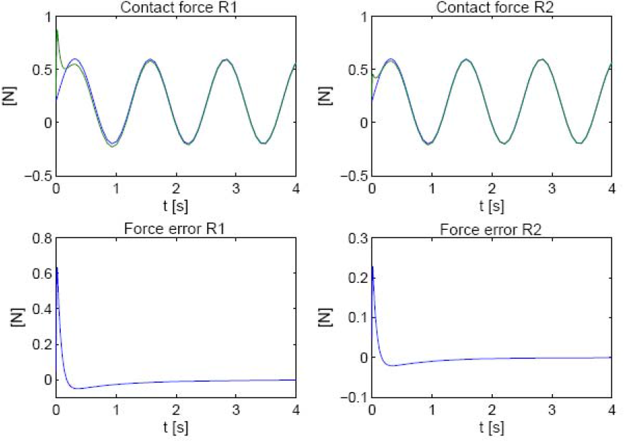
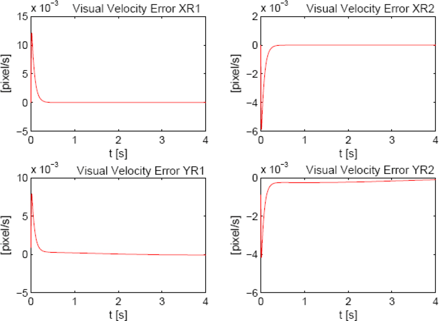
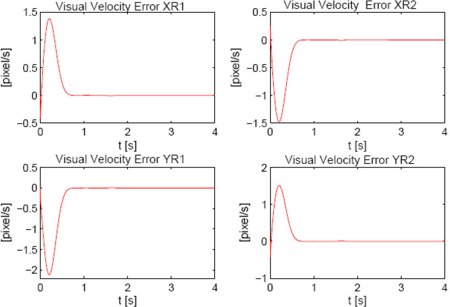
Exponential visual tracking errors for position and velocity are presented in Figures 1 and 2, respectively. The system trajectories converge to an error that can be considered as zero (less than 0.1 pixel error). After a transient response in a few milliseconds in the first joints of the robotic manipulators, the control effort applied to each joint is smooth and chattering free, Fig. 3. Finally, the performance of the contact force and force tracking errors are presented in Fig. 4. As is expected, the simulation results show exponential convergence without any knowledge of i-th robot dynamics and the camera, i.e., the Jacobian ${\stackrel{⌢}{\mathrm{J}}}_{\mathrm{R}\mathrm{i}\mathrm{n}{\mathrm{v}}_2}$ is parameterized in terms of regressor times as parameter vector ${\stackrel{⌢}{\mathrm{m}}}_{\mathrm{i}}.$ Then, the vector is multiplied by a factor to get X% of uncertainty with respect to the nominal value. In these simulations, the desired image-based desired trajectories are defined as follows: ${\mathrm{x}}_{\mathrm{s}{\mathrm{d}}_{\mathrm{i}}}=0,6\left[\mathrm{p}\mathrm{i}\mathrm{x}\mathrm{e}\mathrm{l}\mathrm{s}\right],{\mathrm{y}}_{\mathrm{s}{\mathrm{d}}_{\mathrm{i}}}=0.05-0.03\sin \left(0.5\mathrm{t}\right)\left[\mathrm{p}\mathrm{i}\mathrm{x}\mathrm{e}\mathrm{l}\mathrm{s}\right]$ and ${\lambda }_{{\mathrm{d}}_{\mathrm{i}}}\left(\mathrm{t}\right)=0.2+0.4\sin \left(5\mathrm{t}\right)\left[\mathrm{N}\right]$ , respectively. In addition, the feedback gains used in this experiment are: $\begin{array}{l}{K}_{{\mathrm{d}}_{\mathrm{i}}}=\mathrm{d}\mathrm{i}\mathrm{a}\mathrm{g}\left[10\right],A_{\mathrm{i}}=\mathrm{d}\mathrm{i}\mathrm{a}\mathrm{g}\left[3.8\right],{\xi }_{\mathrm{i}}=\mathrm{d}\mathrm{i}\mathrm{a}\mathrm{g}\left[10\right],\\ b_{\mathrm{i}}=\mathrm{d}\mathrm{i}\mathrm{a}\mathrm{g}\left[0.29\right],{\gamma }_{\mathrm{f}\mathrm{i}}=\mathrm{d}\mathrm{i}\mathrm{a}\mathrm{g}\left[0.0001\right],\\ {\gamma }_{\mathrm{p}\mathrm{i}}=\mathrm{d}\mathrm{i}\mathrm{a}\mathrm{g}\left[0.0001\right],\mathrm{k}=20\end{array}$ .

Figure 1.

Visual position tracking errors for two robot fingers grasping an object.

Figure 2.

Visual velocity tracking errors for two robot fingers grasping an object.

Figure 3.

Smooth control applied to each joint.

Figure 4.

Contact force and force errors applied to the object by each finger.

Finally, we assumed that 90% of parametric uncertainties on ${\stackrel{⌢}{J}}_{{\text{Rinv}}_2}$ exists.

As a second case, a general scheme for free motion and constrained motion through a smooth transition is presented. A smooth transition allows us to avoid an impact regime between the robotic finger and the object, that is, a zero transition velocity from the free motion to constrained motion can be guaranteed. Therefore, impulsive dynamics does not appear and position controller commute stably to position/force controller and vice versa. To ensure that each robot finger approaches on the object surface to a velocity near to zero, it is necessary to change the feedback gain A_i defined in (24) by $A_{\mathrm{i}}\left(\mathrm{t}\right)={\alpha }_{0_{\mathrm{i}}}\frac{{\xi }_{\mathrm{i}}}{1-{\xi }_{\mathrm{i}}+{\delta }_{\mathrm{i}}}$ where ${\alpha }_{0_{\mathrm{i}}}=1+\in$ , for small positive scalar ∊ such that α₀ is close to 1 and 0 < δ ≪ 1. The time base generator ξ_i = ξ_i(t) ∊ C² must be provided by the user so as ξ_i goes smoothly from 0 to 1 in finite time ${\mathrm{t}}_{\mathrm{i}}={\mathrm{t}}_{{\mathrm{b}}_{\mathrm{i}}}$ and ξ_i = ξ_i(t) is a bell-shaped derivative of ξ_i such that ${\xi }_{\mathrm{i}}\left({\mathrm{t}}_0\right)={\xi }_{\mathrm{i}}\left({\mathrm{t}}_{{\mathrm{b}}_{\mathrm{i}}}\right)\equiv 0$ [17]. Once a finite time convergence of position and velocity trajectories is assured in free motion, a stable switching of the closed-loop system to constrained motion is guaranteed.

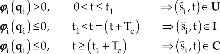
Under the framework presented in the previous sections, the i-th geometric function in these three phases is defined as

$$\begin{array}{l}{\phi }_{\mathrm{i}}\left(q_{\mathrm{i}}\right)\text{ > }0,0\text{ < }\mathrm{t}\le {\mathrm{t}}_1\Rightarrow \left({\stackrel{⌢}{\mathrm{s}}}_{\mathrm{i}},\mathrm{t}\right)∊U\\ {\phi }_{\mathrm{i}}\left(q_{\mathrm{i}}\right)\le 0,{\mathrm{t}}_1\text{ < }\mathrm{t}=\left(\mathrm{t}+{\mathrm{T}}_{\mathrm{c}}\right)\Rightarrow \left({\stackrel{⌢}{\mathrm{s}}}_{\mathrm{i}},\mathrm{t}\right)∊I\\ {\phi }_{\mathrm{i}}\left(q_{\mathrm{i}}\right)\le 0,\mathrm{t}\ge \left({\mathrm{t}}_1+{\mathrm{T}}_{\mathrm{c}}\right)\Rightarrow \left({\stackrel{⌢}{\mathrm{s}}}_{\mathrm{i}},\mathrm{t}\right)∊C\end{array}$$

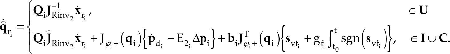
where U is the unconstrained space (Phase 1), I is the transition space (Phase 2), C is the constrained space (Phase 3), t₁ is the contact time which is defined by the user through t_bi and T_c is the contact time which is a very small time period. For free and constrained tasks, Jφ_i+ q_i and Q_i are defined as follows

$$\begin{array}{ll}\mathrm{ }{J}_{{\phi }_{\mathrm{i}}+}\left(q_{\mathrm{i}}\right)=\{\begin{array}{l}0,∊U\\ \nabla {\phi }_{\mathrm{i}}/\Vert {\phi }_{\mathrm{i}}\Vert ,∊I\cup C.\end{array},& Q_{\mathrm{i}}=\{\begin{array}{l}I,∊U\\ I_{{\mathrm{n}}_{\mathrm{i}}}-J_{{\phi }_{\mathrm{i}}+}\left(q_{\mathrm{i}}\right)J_{{\phi }_{\mathrm{i}}}\left(q_{\mathrm{i}}\right),∊I\cup C.\end{array}\end{array}$$

In addition, the noncalibrated nominal reference ${\dot{\stackrel{⌢}{\mathrm{q}}}}_{{\mathrm{r}}_{\mathrm{i}}}$ becomes:

$${\dot{\stackrel{⌢}{\mathrm{q}}}}_{{\mathrm{r}}_{\mathrm{i}}}=\{\begin{array}{l}{Q}_{\mathrm{i}}{J}_{\mathrm{R}\mathrm{i}\mathrm{n}{\mathrm{v}}_2}^{-1}{\dot{x}}_{{\mathrm{r}}_{\mathrm{i}}},∊U\\ Q_{\mathrm{i}}{\stackrel{⌢}{J}}_{\mathrm{R}\mathrm{i}\mathrm{n}{\mathrm{v}}_2}^{}{\dot{x}}_{{\mathrm{r}}_{\mathrm{i}}}+J_{{\phi }_{\mathrm{i}}+}\left(q_{\mathrm{i}}\right)\left\{{\dot{p}}_{{\mathrm{d}}_{\mathrm{i}}}-{\mathrm{E}}_{2_{\mathrm{i}}}\Delta p_{\mathrm{i}}\right\}+b_{\mathrm{i}}{J}_{{\phi }_{\mathrm{i}}+}^{\mathrm{T}}\left(q_{\mathrm{i}}\right)\left\{s_{\mathrm{v}{\mathrm{f}}_{\mathrm{i}}}+{\mathrm{g}}_{{\mathrm{f}}_{\mathrm{i}}}{\displaystyle {\int }_{{\mathrm{t}}_0}^{\mathrm{t}}\text{sgn}\left(s_{\mathrm{v}{\mathrm{f}}_{\mathrm{i}}}\right)}\right\},∊I\cup C.\end{array}$$

Therefore, the uncertain visual error manifold is defined as

$${\stackrel{⌢}{\mathrm{s}}}_{\mathrm{i}}=\{\begin{array}{l}{Q}_{\mathrm{i}}\left(J_{\mathrm{R}\mathrm{i}\mathrm{n}{\mathrm{v}}_2}^{}{\dot{x}}_{{\mathrm{s}}_{\mathrm{i}}}-{\stackrel{⌢}{J}}_{\mathrm{R}\mathrm{i}\mathrm{n}{\mathrm{v}}_2}^{}{\dot{x}}_{{\mathrm{r}}_{\mathrm{i}}}\right),∊U\\ Q_{\mathrm{i}}\left(J_{\mathrm{R}\mathrm{i}\mathrm{n}{\mathrm{v}}_2}^{}{\dot{x}}_{{\mathrm{s}}_{\mathrm{i}}}-{\stackrel{⌢}{J}}_{\mathrm{R}\mathrm{i}\mathrm{n}{\mathrm{v}}_2}^{}{\dot{x}}_{{\mathrm{r}}_{\mathrm{i}}}\right)-J_{{\phi }_{\mathrm{i}}+}^{\mathrm{T}}\left(q_{\mathrm{i}}\right)\left\{\Delta {\dot{p}}_{\mathrm{i}}+{\xi }_{2_{\mathrm{i}}}\Delta p_{\mathrm{i}}+{\mathrm{b}}_{\mathrm{i}}{s}_{\mathrm{v}\mathrm{x}{\mathrm{f}}_{\mathrm{i}}}\right\},∊I\cup C.\end{array}$$

Then, using (42) the open loop error equation for free and constrained tasks is given as in equation (27), i.e.,

$$H_{\mathrm{i}}\left(q_{\mathrm{i}}\right){\dot{\stackrel{⌢}{\mathrm{s}}}}_{\mathrm{i}}+C_{\mathrm{i}}\left(q_{\mathrm{i}},{\dot{q}}_{\mathrm{i}}\right){\stackrel{⌢}{\mathrm{s}}}_{\mathrm{i}}=u_{\mathrm{i}}-Y_{\mathrm{c}\mathrm{o}\mathrm{n}{\mathrm{t}}_{\mathrm{i}}}{\stackrel{⌢}{m}}_{\mathrm{i}}+J_{{\phi }_{\mathrm{i}}+}^{\mathrm{T}}\left(q_{\mathrm{i}}\right){\lambda }_{\mathrm{i}}+u_{{\mathrm{d}}_{\mathrm{i}}}$$

(43)

where

$$J_{{\phi }_{\mathrm{i}}+}^{\mathrm{T}}\left(q_{\mathrm{i}}\right){\lambda }_{\mathrm{i}}=\{\begin{array}{l}0,∊U\\ J_{{\phi }_{\mathrm{i}}+}^{\mathrm{T}}\left(q_{\mathrm{i}}\right){\lambda }_{\mathrm{c}\mathrm{o}\mathrm{n}{\mathrm{t}}_{\mathrm{i}}},∊I\cup C.\end{array}$$

with ${\lambda }_{\mathrm{c}\mathrm{o}\mathrm{n}{\mathrm{t}}_{\mathrm{i}}}$ is now the contact force. Finally, the neuro-adaptive law is given as

$$u_{\mathrm{i}}=\{\begin{array}{l}-K_{{\mathrm{d}}_{\mathrm{i}}}{\stackrel{⌢}{\mathrm{s}}}_{\mathrm{i}}+x_{\mathrm{i}}^{\mathrm{T}}{\stackrel{⌢}{w}}_{\mathrm{i}},∊U\\ -K_{{\mathrm{d}}_{\mathrm{i}}}{\stackrel{⌢}{\mathrm{s}}}_{\mathrm{i}}+x_{\mathrm{i}}^{\mathrm{T}}{\stackrel{⌢}{w}}_{\mathrm{i}}+J_{{\phi }_{\mathrm{i}}+}^{\mathrm{T}}\left(q_{\mathrm{i}}\right)\left[-{\lambda }_{{\mathrm{d}}_{\mathrm{i}}}+{\eta }_{\mathrm{i}}\Delta f_{\mathrm{i}}\right]\\ +{\gamma }_{{\mathrm{F}}_{\mathrm{i}}}{J}_{{\phi }_{\mathrm{i}}+}^{\mathrm{T}}\left(q_{\mathrm{i}}\right)\left[\tanh \left({\mu }_{\mathrm{i}}{s}_{\mathrm{v}{\mathrm{f}}_{\mathrm{i}}}\right)+{\eta }_{\mathrm{i}}{\displaystyle {\int }_{{\mathrm{t}}_0}^{\mathrm{t}}\mathrm{sgn}\left(s_{\mathrm{v}{\mathrm{f}}_{\mathrm{i}}}\right)}\right],∊I\cup C.\end{array}$$

and

$${\dot{\stackrel{⌢}{\mathrm{w}}}}_{\mathrm{i}}=\{\begin{array}{l}-{\Gamma }_{\mathrm{i}}{X}_{\mathrm{i}}^{\mathrm{T}}{\stackrel{⌢}{\mathrm{s}}}_{\mathrm{i}},∊U\\ -{\Gamma }_{\mathrm{i}}{X}_{\mathrm{i}}^{\mathrm{T}}{\stackrel{⌢}{\mathrm{s}}}_{\mathrm{i}},∊I\cup C.\end{array}$$

where $K_{{\mathrm{d}}_{\mathrm{i}}},{\gamma }_{{\mathrm{F}}_{\mathrm{i}}},{\eta }_{\mathrm{i}},{\mu }_{\mathrm{i}},{\lambda }_{{\mathrm{d}}_{\mathrm{i}}},{\Gamma }_{\mathrm{i}}$ have the same dimensions as defined in equations (30) and (31) respectively.

From the previous definitions for transition tasks, we proceed to describe the task. Consider two rigid planar robots as fingers which are not grasping the object initially. Then, from any initial condition the end-effector of the i-th robot finger will follow a desired trajectory (cubic polynomial) in finite time t_bi (free control) under 75% of parametric uncertainty on ${\stackrel{⌢}{J}}_{\mathrm{R}\mathrm{i}\mathrm{n}{\mathrm{v}}_2}$ . Once stable contact is achieved, the position controller commutes to a force/position controller (constrained motion). Then, ${\lambda }_{\mathrm{d}\mathrm{i}}=2\sin \left(5\mathrm{t}\right)\left[\mathrm{N}\right],{\mathrm{x}}_{\mathrm{s}{\mathrm{d}}_{\mathrm{i}}}=0.3482\left[\mathrm{p}\mathrm{i}\mathrm{x}\mathrm{e}\mathrm{l}\mathrm{s}\right]$ and ${\mathrm{y}}_{\mathrm{s}{\mathrm{d}}_{\mathrm{i}}}=0.4203-0.1\mathrm{s}\mathrm{e}\mathrm{n}\left(0.2\mathrm{t}\right)\left[\mathrm{p}\mathrm{i}\mathrm{x}\mathrm{e}\mathrm{l}\mathrm{s}\right]$ represent the force and desired visual trajectories in constrained motion under 75% of parametric uncertainty on ${\stackrel{⌢}{J}}_{\mathrm{R}\mathrm{i}\mathrm{n}{\mathrm{v}}_2}.$ Visual tracking errors for free and constrained motion are shown in Fig. 5. The impulse response between position and force controller commutation is avoided, as shown in Fig. 6. Instead, the performance of the control signal is smooth and chattering free. Additionally, in Fig.8 we can observe that the change in the velocity before and after collision, is the same, i.e. $\dot{q}\left({\mathrm{t}}_{\mathrm{b}}\right)=\dot{q}\left({\mathrm{t}}_{\mathrm{b}}+\mathrm{h}\right),$ with h > 0 so that acceleration is analytic. On the other hand, Fig. 7 shows that before t ≤ 1.5[s], the contact force is zero, however, for t>1.5[s] the force converges to a desired value after a few seconds, i.e., the robot grasps an object rigidly. The feedback gains used in this experiment are:

Figure 5.

Visual position tracking errors for transition tasks.

Figure 6.

Smooth control input applied to each joint.

Figure 7.

Contact force and force error applied to the object by each finger.

Figure 8.

Visual velocity tracking errors for transition tasks.

$$\begin{array}{l}{K}_{{\mathrm{d}}_{\mathrm{i}}}=\mathrm{d}\mathrm{i}\mathrm{a}\mathrm{g}\left[10\right],A_{\mathrm{i}}=\mathrm{d}\mathrm{i}\mathrm{a}\mathrm{g}\left[3.8\right],{\xi }_{\mathrm{i}}=\mathrm{d}\mathrm{i}\mathrm{a}\mathrm{g}\left[10\right],\\ b_{\mathrm{i}}=\mathrm{d}\mathrm{i}\mathrm{a}\mathrm{g}\left[0.29\right],{\gamma }_{\mathrm{f}\mathrm{i}}=\mathrm{d}\mathrm{i}\mathrm{a}\mathrm{g}\left[0.0001\right],\\ {\gamma }_{\mathrm{p}\mathrm{i}}=\mathrm{d}\mathrm{i}\mathrm{a}\mathrm{g}\left[0.0001\right],\mathrm{k}=20.\end{array}$$

Finally, we have not obtained a systematic procedure to tune the control gains basically because of the nonlinear nature of the closed-loop system. Thus, the feedback gains are tuned on a trial-and-error-basis, according to the interplay of each gain in the closed-loop system.

6. Conclusions

A neuro-visual servoing controller which guarantees image-based tracking of constrained multiple robot arms subject to parametric uncertainty is proposed. Exponential convergence in the visual force/position subspaces is guaranteed, even when neither robot parameters nor camera parameters are known. The main feature of our scheme is the ability to fuse the image coordinates/visual velocities and contact forces in orthogonal complements. The neural network control loop compensates for DAE dynamics, while an inner piecewise continuous sliding mode control loop adds the missing effort to induce sliding modes. Numerical simulations allow us to validate our proposed scheme through two significant applications: two robotic manipulators grasping a rigid object, and two robotic fingers executing tasks that involve changing dynamics and impact regime.