
Abstract
The inertial and friction parameters of a robot are used in the development and evaluation of model-based control schemes and their accuracy is related directly to the performance. These parameters can also be used for a realistic simulation, which may be useful before implementation of new control schemes. In principle, the numerical value of the parameters could be obtained via CAD analysis, but inevitably assembly and manufacturing errors exist. Direct measurement is not a realistic option because the complex nature of the system involves intense, time-consuming effort. Alternatively, we can deduce the values of the parameters by observing the natural response of the system under appropriate experimental conditions, i.e., by using identification schemes, which is an efficient way. This paper presents the experimental evaluation of five identification schemes used to obtain the inertial and friction parameters of a three-degrees-of-freedom direct-drive robot. We assume that the inertial and friction parameters are totally unknown but, by design, the dynamic model is fully known, as in many practical cases. We consider the schemes based on the dynamic regression model, the filtered-dynamic regression model, the supplied-energy regression model, the power regression model and the filtered-power regression model. This paper presents a comparison between experimental and simulated robot response, which enables us to verify the accuracy of each regression model.
1. Introduction
Model based control schemes for robot manipulators, such as computed-torque control, PD+ control and PD control with computed feedforward, require accurate information on the robot dynamics. An accurate system-identification process is a crucial step required to improve the performance of such control schemes, while enabling a realistic robot simulation. Dynamic parameters can include the mass, the inertia tensor, the length and the centre of gravity of each link, as well as the friction coefficients. The value of such parameters is, in general, not known in advance, even by the robot manufacturer. Often, the only model available is the kinematic model of the manipulator, while the dynamic model is not well known. Direct measurement of the dynamic parameters is not a realistic option, because assembling and disassembling the robot is not an easy task. Also, a CAD-based model is insufficient because inevitably assembly and manufacturing errors exist. Therefore, identification techniques for robot manipulators are particularly attractive to determine the dynamic parameters of robot manipulators when a direct measurement of the parameters of each link is not a viable solution. In this context, an experimental identification scheme is the most practical alternative.
In robotic identification, commonly the ordinary nonlinear differential equations describing the dynamical model of a manipulator with revolute and prismatic joints, are expressed in a linear fashion with respect to the unknown dynamic parameters. Although friction is a complex nonlinear phenomenon, a friction model consisting of only Coulomb and viscous friction is an acceptable simplification for many robotics applications. Also, by using this friction model, the friction phenomenon can be described in a linear scheme with respect to the unknown Coulomb and viscous-friction parameters, which is consistent with the linear-model structure.
The linear-model structure is used particularly in a few identification schemes based on regression models. For example, early work requiring joint-acceleration information within the regression model is referred to as the dynamic-regression model or the differential-regression model [1, 2]. The first approach requiring joint-acceleration, referred to as the filtered-dynamic regression model, was proposed by Hsu [3].
The total energy applied to robot manipulators can be described in a linear-model structure by a combination of the dynamic and friction parameters, according to the principle of energy conservation. Such a form was used to propose the supplied-energy regression model [4], also known as the integral model [1]. Both the filtered dynamic model and the energy model are regression models independent of joint acceleration. It is well known that the supplied energy model leads to a scalar prediction error while the filtered dynamic model leads to a vector-prediction error.
Another regression model based on the principle of energy conservation was proposed by Reyes and Kelly [5]. That regression model was referred to as the filtered-power model and was derived indirectly from the supplied-energy model proposed by Gautier and Khalil [4]. The supplied-energy model involves the integral of the power while the filtered-power model contains a low-pass filter of the power. The filtered-power model can be obtained by the differentiation with respect to time of the supplied-energy model after applying a low-pass filter.
In the literature there are many references related to the identification of robots. However, during the last decade only a few works include an experimental comparison of the various regression models. In earlier papers we can read about the experimental comparison between filtered-dynamic and supplied-energy models on a direct driven, two link robot [1]. As shown in this reference, the filtered-dynamic model has advantages with respect to the supplied-energy model. In [2], both regression models were tested on a non direct-drive robot and it is concluded that the filtered-dynamic model has advantages over the supplied-energy model.
Reyes and Kelly [5] presented a comparison, based on experimental evidence, between three regression models tested on a two-degrees-of-freedom direct-drive robot. In this work, the tested regression models were the filtered-dynamic, the supplied-energy and the filtered-power models. These schemes belong to the hybrid identification philosophy [6], i.e., the estimation is performed by a recursive estimator while the regression model is formulated in continuous time. They concluded that the filtered-dynamic scheme provides better parameter estimates with increased complexity in the implementation. The other regression schemes reduce the computational process and are more suitable for real-time implementation. Also if Coulomb friction is present, the filtered-power model offers advantages over the approach based on the supplied-energy model. Note that in [5], the identified parameters were compared to those obtained by measuring the link parameters and later used to reproduce simulated results which are compared with current experimental data. A difference in behaviour was observed.
Recent approaches in dynamic-parameter identification consider direct and indirect identification processes. In the indirect identification process, system parameters are individually identified in multiple steps. The identification trajectories usually consist of one or two joints motions at a time, which can be generated by simple controllers. Examples of such identification methods can be found in [7, 8, 9].
On the other hand, direct identification methods are based on a single motion trajectory that excites all the parameters of the robot dynamics. The challenging part of this method is the design of the identification trajectory that leads to an optimum estimation of the system parameters. The trajectory optimization problem is addressed in several research works such as [10, 11, 12, 13].
In [14] the authors present an overview of the dynamic parameter identification of robots. They classify methods as off-line and on-line and also discuss trajectory optimization. In [15] we can find a comparison between two methods to estimate only the inertial parameters of an industrial robot: the least squares method and particle swarm optimization. They conclude that the accuracy of the estimated parameters depends on the estimation methods, the measurement accuracy and the selection of efficient exciting trajectories. We can find another interesting proposal, for example in [16], which presents a method to estimate individual parameter values based on a dependency analysis of the regressors based on measured motion trajectory data. In [17] the authors propose a new method for parameter identification that only uses the force/torque measurement. The method is based on a closed-loop simulation using the direct dynamic model, the same structure of the control law and the same reference trajectory.
In this paper a procedure to obtain the parameter identification of a robot manipulator is presented. Therefore, the main goal of this work consists of designing an experimental comparison of off-line robot-dynamics estimation between the following five identification schemes: the dynamic model, the filtered-dynamic model, the supplied-energy model, the power model and the filtered-power model. Such hybrid identification schemes can be considered as direct identification processes. In these schemes, the same estimator, the recursive least-squares algorithm, is implemented. We assume that the dynamical and friction parameters of our experimental direct-drive arm are unknown. In order to validate the parameter values obtained from the best regression scheme, we compare open loop joint positions of the actual robot with simulations, using a robot model with these identified parameters. Another procedure for validating the identified parameters consists of reproducing the applied torque from the torque computed with dynamical model. This comparison is also presented. The experimental platform used is a three-degrees-of-freedom direct-drive robot and the complete dynamic model is developed and presented in explicit form. In order to obtain the complete dynamic model, an approach based on Lagrange's equations of motion is used. In technical literature related to robot identification, there are works that includes as case studies a two-degrees-of-freedom direct-drive robot, such as [5, 17, 18, 19, 20]. A few works includes as case studies an anthropomorphic three-degrees-of-freedom direct-drive robot, or the first three-degree- of-freedom of a more complex robot, also a small number of them exhibit the explicit model or show the procedure to obtain it. Among these works, some features of mass distribution were assumed in order to simplify the analysis and get an approximate-simplified model. Examples of papers that include experimental results using a three-degree-of-freedom robot are [12, 13, 15, 21, 22]. In the case of our experimental robot, the model was developed without assuming any shapes in the links, i.e., the links are modelled as a general rigid body, as a result a complete dynamic model was obtained.
2. Dynamical model for direct drive robots
The dynamical analysis of the bodies in movement determines a relationship between applied generalized-external forces and the motion of the object; in robotics such relationships are implied by joint torques/forces applied by the actuators and the motion of the robot. The motion of the robot is described by the joint positions, joint velocities and joint accelerations of the robot arm as a function of time. Robot manipulators have complex nonlinear dynamics. However, fortunately robot dynamic models can be obtained in closed form, in a straightforward way by using, for example, Lagrange's equations of motion. The use of Lagrange's equations requires the notion of two important concepts: kinetic and potential energies.
It is well known that the dynamics of a serial n-link rigid robot can be written as:

where

where:

It is well known that it is possible to define combinations of inertial parameters such that the dynamical model (1) is linear with respect to each combination. The complete set of parameters describing the mass distribution is referred to as barycentric parameters. The dynamic model contains only a few independent combinations of these barycentric parameters and the friction parameters, as follows:

where
3. Parameter identification
In this section, we present five different regression models to obtain the identification parameters of a three-degrees-of-freedom robot. All regression models use the recursive least-squares approach. A short overview of the recursive least-squares method and the formulation of regression models is presented in the following.
3.1 Recursive least-squares algorithm
The least-squares method is a standard technique used to obtain an approximate solution for over-determined systems. The least-squares method computes the minimum of a square errors sum; the error is defined by the difference between measured data and the computed data using the mathematical model, in our case the dynamical model of robots. If the model has the property of being linear in the parameters then the method is particularly simple. Let us consider the following regression model:

where
The estimated value of vector


where the prediction error

3.2 Dynamic and Filtered-dynamic regression models
The robot dynamics model (1) describes the relationship between torques applied to the joints and the resulting motion of the links. The representation of the robot dynamics model given in (4), which relates joint torques with the unknown dynamic parameters is referred to as the differential regression model [1, 23, 24] and can be written as:

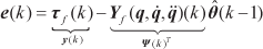
to coincide with the above notation in Section 3.1. The prediction error for the dynamic regression model can be written as

In this regression model, in order to compute the elements of the regressor matrix
The principal idea is to filter both sides of the differential regression model (9) by a stable strictly-proper filter. A simple first order filter has been considered in the literature. The filter has been denoted by its transfer function:

where λ > 0 and s stands for the differential operator.
Therefore, the filtered dynamic regression model can be written as:

where:

Notice that the measurement of joint acceleration
3.3 Supplied-energy regression model
The supplied-energy regression model introduced by Gautier and Khalil [4] is based on the principle of energy conservation. The work of the non-conservative forces applied to a system is equal to the change of the total energy of the system:

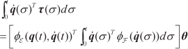
Using the property of linearity in the parameters of the robot's total energy [5] the principle of the conservation of energy (15) and assuming that the total energy at the instant zero is null, we obtain the supplied-energy regression model [4]:
which is linear in the barycentric and friction parameters. Note that, in order to compute the regressor matrix, the measurement of joint acceleration
The prediction error of the supplied-energy regression model to be used in the recursive least-squares algorithm can be written as:

where h denotes the sampling period.
3.3 Power and Filtered-power regression models
By using the supplied energy regression model (16) we can compute the power applied to the manipulator. The power applied to the robot is the instantaneous change in the total supplied energy:

and the prediction error for the power regression model can be written as:

This model presents the drawback of requiring the joint acceleration measurement in order to compute the matrix regressor.
The filtered-power regression model was proposed by Reyes and Kelly [5] based on the supplied energy regression model and overcomes this shortcoming. The principal idea is to filter both sides of the power model (18) via a stable, strictly-proper filter. Again the first order filter described in (11) can be considered. By applying the filter to both sides of (18) we obtain the filtered-power regression model:

The above model is linear in the barycentric and friction parameters. Also, in order to compute the regressor matrix, the measurement of joint acceleration

4. Experimental Platform
The experimental results are presented on an anthropomorphic direct drive robot which was designed and built at the Robotics laboratory of Benemérita Universidad Autónoma de Puebla (BUAP). The three-degree-of-freedom robot called “Rotradi”, consists of three 6061 aluminium links actuated by brushless direct-drive servo actuators in order to drive the joints without gear reduction. The motors used in “Rotradi” are DM-1050A, DM-1150A and DM-1015B models from Parker Compumotor, for the base, the shoulder and elbow joints respectively. The servos are operated in torque mode, which means that the motor acts as a torque source and they accept an analogue voltage as a reference of torque signal. Servo actuator features are shown in Table 1. The robot system has a device designed for reading the encoders and generates reference voltages, which is a motion control board of Precision MicroDynamics Inc. Control algorithms are written in C code and run in real time with a 2.5 ms sample period on a Pentium-1 at 166 MHz.
Robot arm servo actuators

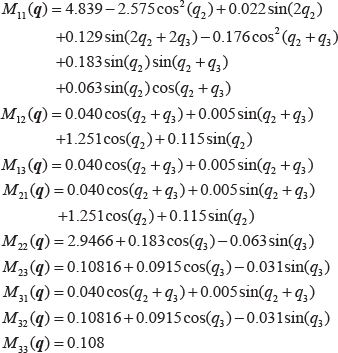
The complete dynamics model of our experimental arm has been developed considering that the links don't have a specific shape, i.e., the links are considered as rigid bodies without a specific mass distribution. The elements of the inertia matrix are given by:

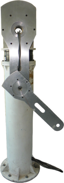
Experimental robot “Rotradi”
The elements of Coriolis and Centripetal torque vectors are given by:

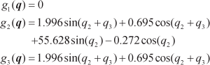
The elements of gravitational torque vectors are given by:
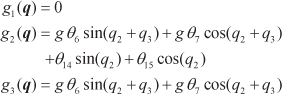
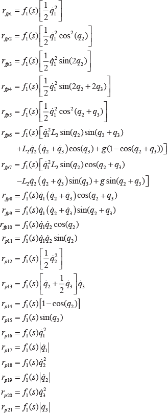
and the elements of friction torque vectors are given by:

where the time-invariant barycentric and friction parameters θ
i
,i=1,…,21 are given by:

In identification schemes the choice of input trajectories for exciting the robot is very important. A good selection of trajectories leads to an accurate model-parameter determination. For our identification problem the required trajectories are referred to as weakly persistent excitation trajectories. The selection of this kind of trajectory is not trivial and due to its complexity is not addressed in this paper.
Guided by practical experience, we propose a procedure to tune the torque trajectory. The mathematical structure of the torque trajectory can be given by:
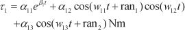


where:

The excitation trajectory for each joint is tuned considering many experiments such that:
In order to obtain the adequate amplitude of the torque trajectory, parameters α1i,α2j,α3i,w1i,w2j, β
i
∈
Extensive experiments were carried out with several torque trajectories that contain sinusoidal functions with different frequencies to excite the system. The best results of parameter identification were obtained by using the following trajectories:

where ran1 takes random values with uniform distribution within the interval (-5,…,45) degrees, ran2 within (–35,…,35) degrees, ran3 within (–50,…,0) degrees, ran4 within (40,…,100) degrees, ran5 within (5,…,35) degrees and ran6 within (–30,…,30) degrees.
It is important to note that the resulting motion of the robot covers the following aspects:
Good coverage of the workspace improves the information content of the measurements as well as the accuracy of the parameter estimates. High accelerations are required to accurately estimate the moments and products of inertia. Joint velocity must be within the actuator's bandwidth and lower than the lowest resonance frequency of the robot structure. The structural flexibilities of the robot are excited close to the lowest resonance frequency. The excitation of flexible modes is disadvantageous because they are not accounted for in the rigid-body robot model.
The robot arm has incremental encoders to measure joint position; each encoder has a 1,024,000 cpr resolution (see Table 1). The joint velocity was computed by using a standard backwards difference algorithm applied to the position measurement. In the experiments the arm started its motion according to the following initial conditions:
The aforementioned regression schemes are presented in detail in the following sections.
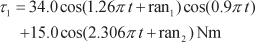
4.1 Dynamic regression model
The prediction error for the dynamic regression model is described in (10). For our robot arm, the regressor matrix is given by:

where:
The value of items not shown here is zero.
4.2 Filtered-dynamic regression model
The prediction error for the filtered-dynamic regression model is described by (14). For our robot arm, the regressor matrix is given by:

where:
where
Since the measured values of joint torques, positions and velocities hold constant between sampling instants, filters can be implemented in discrete form. Actually
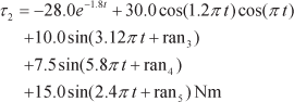
4.3 Supplied-energy regression model
The prediction error of the supplied-energy regression model is given by Equation (17). For our robot arm, the regressor matrix is given by

where:

The integrals have been implemented with standard trapezoid-type integration rules.
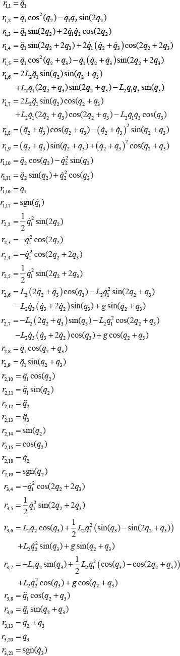
4.4 Power regression model
The prediction error of the power regression model is defined in (19). For our robot arm, the regressor matrix is given by:

where

4.5 Filtered-power regression model
The prediction error of the filtered-power regression model was defined in (21). For our robot arm, the regressor matrix is given by:
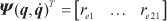
where:
The filters f1(s) and f2(s) shown in the above expressions are implemented in the same way as in the filtered dynamic model.
5. Experimental results
In this section we compare the experimental results obtained from the identification schemes described in Section 4. The best results were obtained with the filtered-dynamic model. This conclusion is based on the comparison between the experimental data and the simulated dynamics behaviour with the identified parameter values. We define the error between the simulated and experimental positions as

and then compute the norm ‖qerror i‖2; the numerical values are shown in Table 2. The cutout frequency for the filtered schemes was chosen as λ = 9.11 rad/s. This value was selected by testing several frequencies; the one enabling a closer approximation between simulated dynamics and real response was chosen.
Norm 2 ‖·‖ of error between experimental and simulated positions

Table 3 shows the results for different identification schemes, the dimensional units are implicit for all data parameters. As mentioned above, the measuring instrument for the experiment is an incremental encoder used to measure position, while velocities and accelerations are computed using numerical differentiation. Each encoder has 1,024,000 cycles-per-revolution, enabling a numerical accuracy of 6.1359×10⁻⁶[rad/cycle]; for this reason the results are presented to the sixth digit of precision.
Identified parameters

Table 4 shows the standard variation with respect to values obtained by using the filtered-dynamic model scheme. The filtered-power regression model presents less variation in parameter values as compared to the filtered-dynamic regression model; the power regression model presents higher variation with respect to the filtered dynamic regression model followed by the supplied energy regression model. However, the numerical values of some parameters have a greater influence on the dynamics of the robot than others.
Variation of parameter values

Figure 2. shows the evolution of the parameter vector θ with respect to time. Parameter θ14 has been scaled by factor 0.1 for presentation purposes, i.e., to show the values at a scale similar to the rest of the parameters.

Evolution of parameter vector θ with respect to time
An important property of the least-squares algorithm is that convergence is guaranteed when the weakly persistent exciting condition is satisfied [25]. This property can be written as:

which are directly related with:

In order to show the convergence of the recursive least-squares algorithm we have included a plot with the evolution of the covariance matrix

Evolution of the covariance matrix eigenvalues
A proof that validates the parameter values obtained with regression schemes consists of comparing the open loop responses of the actual robot with simulations using the robot model together with the identified values. In our case, the regression model with the best simulation response, as compared with actual robot response, was the filtered-dynamic regression model. A 4/5 order Runge-Kutta algorithm implemented in Matlab 2009 was used in simulations. We also used trajectories (30)–(32) in order to produce open loop responses in the base, shoulder and elbow respectively. Simulated and actual robot responses are shown in Figure 4.

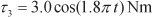
In a technical bibliography it is common to show a comparison between joint torque and the computed torque using a dynamic model of the robot (1). Identification schemes are used to compute dynamic-parameter values for the purpose of applying advanced control laws in manipulator robots. Advanced control laws depend on the dynamic model and their parameter values, for example, computed-torque control. In our case, we show in Figure 5 a comparison between input and computed torques, using trajectories (30)–(32).

In order to compute the torque value the experimental values of positions, velocities and accelerations were used. Only positions are measured directly. Velocities and accelerations are computed via numerical differentiation. It is well known that such numerical processes can induce noise in data torque computation and this is reflected in plots. Another reason could explain the noise in the plots: by design, input trajectories (30)-(32) have a noisy phase.
The dynamical model using numerical values of parameters obtained with the filtered-dynamic regression model (see Table 3) and L2 = 0.45m can be written as follows: the elements of the inertia matrix are given by:
the elements of the Coriolis and Centripetal torque vectors are given by:

the elements of the gravitational torque vectors are given by:
and the elements of friction torque vectors are given by:

In order to strengthen the validity and accuracy of the estimated parameters, we performed an experimental test in open-loop with the robot manipulator. In this experiment, if the measured response is similar to the simulated response then evidence exists on the accuracy of the estimated parameters, but not a definite proof. The test consists of applying different excitation trajectories. The excitation trajectories are as follows:


The actual robot and simulation responses are shown in Figure 6. As shown, both responses are similar but not identical, which means that the robot has not been perfectly characterized. Achieving a perfect match is unrealistic as it implies a perfect model and also that complex phenomena, such as friction, correspond exactly to the proposed representation. In this case, the mathematical description of the phenomena is not unique and is difficult to model in practice. As mentioned above, the best results obtained from a large number of experiments, are presented.

Experimental and simulated responses
The torques applied to the joints and the torques computed by the dynamical model are shown in Figure 7. The computed torque is noisy because velocities and accelerations have been computed using a numerical procedure.
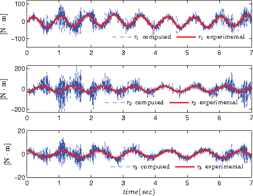
Input and computed torques
7. Conclusion
In this paper we have presented the experimental evaluation of five direct identification schemes to determine the dynamic parameters for a three degrees-of-freedom direct-drive robot. The regression models are: dynamic, filtered-dynamic, supplied-energy, power and filtered-power models.
All identification schemes are based on recursive least-squares algorithms with five regression models.
We consider that the filtered dynamic model scheme presented the best results in the estimating the parameters. This is because the parameters obtained with this regression model can reproduce the experimental response in the simulation of an open-loop experiment. This is shown in Table 2 which contains the numerical values of the quantization error. Table 4 shows the standard variation with respect to the values obtained by using the filtered-dynamic model scheme. The filtered-power regression model presents less variation in parameter values as compared to the filtered-dynamic regression model; the power regression model presents a high variation with respect to the filtered-dynamic regression model followed by the supplied energy regression model. It can be explained if taking into account that the joint velocity and the joint acceleration are estimated by using a numerical procedure. To compute the power regression model, the measurements of joint acceleration are needed and the noise induced in this numerical procedure reduces the quality of the estimation algorithm. However, the numerical value of some parameters has a greater influence on the dynamics of the robot than others. The reproduction of the experiment via simulation enables the determination of the quality of the estimation procedure.
The explicit dynamic model of a three-degrees-of-freedom robot was presented. In order to get the dynamic model an approach based on Lagrange's equations of motion was used. Details of the kinetic and potential energy of all links are presented in the Appendix section. The aim of showing the dynamic model is to make it available for reference, for students and researches. The kinematic configuration of our experimental platform is similar to the first three links of various industrial robots. The explicit model can be used in model based control schemes for robot manipulators.