The parameter identification of the autonomous underwater vehicle based on multi-innovation least squares identification algorithm

Abstract

An accurate model is important for the engineer to design a robust controller for the autonomous underwater vehicle. There are two factors that make the identification difficult to get accurate parameters of an AUV model in practice. Firstly, the autonomous underwater vehicle model is a coupled six-degrees-of-freedom model, and each state of the kinetic model influences the other five states. Secondly, there are more than 100 hydrodynamic coefficients which have different effects, and some parameters are too small to be identified. This article proposes a simplified six-degrees-of-freedom model that contains the essential parameters and employs the multi-innovation least squares algorithm based on the recursive least squares algorithm to obtain the parameters. The multi-innovation least squares algorithm leverages several past errors to identify the parameters, and the identification results are more accurate than those of the recursive least squares algorithm. It collects the practical data through an experiment and designs a numerical program to identify the model parameters. Meanwhile, it compares the performances of the multi-innovation least squares algorithm with those of the recursive least squares algorithm and the least square method, the results show that the multi-innovation least squares algorithm is the most effective way to identify parameters for the simplified six-degrees-of-freedom model.

Introduction

When facing the uncertain ocean environment, it is necessary to design an advanced controller for the autonomous underwater vehicle (AUV) based on the accurate model. Accurate AUV model plays a fundamental role in many applications such as vehicle dynamics simulation, navigation, controller design, fault detection, and diagnosis. ^{1 –3} In the identification of ship maneuvering motion, a dynamic model is typically selected. However, the dynamic model is complex since of highly nonlinear and strong intercoupling characteristics. It is a challenging task to estimate the hydrodynamic coefficients based on the training data measured from the field experiments of the AUV. ⁴

Usually, the model identification needs a lot of experimental data to estimate the parameters, and researchers leverage sufficient data to improve the identification performances. To get data under different conditions, the AUV is programmed to perform a series of maneuvers and sends back data measured by the onboard sensors. ⁵ Traditionally, the captive model test obtains the identification data by performing the ship maneuvers based on the sophisticate facilities such as towing tanks, rotating arms, and planar motion mechanism. ^6,7 These maneuvers can also be simulated by computational fluid dynamics (CFD), but the accuracy of CFD is closely related to the numerical settings. ^8,9 Although estimation with empirical formulas is the most practical and convenient method, it cannot guarantee the identification accuracy. ^10,11 As a widely used modeling method, system identification (SI) uses the measurements of input and output variables to model dynamic systems. ¹² SI based on the free-running test provides a practical and efficient way that requires low experiment time and cost.

According to the SI theory, some classic methods, such as neural networks, ^{13 –15} support vector machines, ^16,17 frequency domain identification, ^18,19 and time domain identification, are used to model the dynamic systems. Usually, the time domain identification method is used to optimize the hydrodynamic coefficients of AUV. The Kalman filtering (KF), ^20,21 particle swarm optimization (PSO), ^22,23 and least square (LS) method ²⁴ are the commonly used methods in practice. In general, these methods aim to identify the parameters by minimizing the error between the desired and the actual outputs. However, these techniques have some problems such as huge amount of computation and poor identification performance. And some modified methods are proposed to improve the performances. Sabet et al. ²⁵ employed the extended Kalman filter (EKF), cubature Kalman filter (CKF), and transformed unscented Kalman filter (TUKF) to identify the parameters that have the highest effects of the modeling error, respectively, and the results showed that the TUKF had the best performances since it solved the nonlocal sampling problem and the linearization problem of the CKF and EKF. Dai et al. ²⁶ introduced a novel PSO algorithm named OPSO to identify the hydrodynamic parameters of motions. However, it is difficult to choose the parameters of PSO since they are set according to the specific problems, application experience, and numerous experiment tests. In addition, the PSO is easy to be trapped into the local optima and it is necessary to design an effective strategy to balance the global exploration and local exploitation. Ridao et al. ²⁷ compared the direct LS identification method with the integral LS identification method in an off-line identification test, and the results showed that the latter is more effective to get an accurate model of the AUV.

However, some research studies have pointed out that the above-mentioned methods present some limitations. Since there are many uncertain damping terms in the AUV model, the convergence rate and accuracy of the algorithms are not the same as the desired. ²⁸ In addition, only a few studies have considered the small sample estimation of the AUV parameters. To deal with these problems, we use a multi-innovation least squares (MILS) identification algorithm to identify the parameters of the AUV. The MILS is an improved algorithm based on the recursive least squares (RLS) algorithm. The RLS is the basic method in SI, and its accuracy and convergence are relative to the amount of useful experimental data. As a modified algorithm of the RLS, the MILS algorithm improves the identification accuracy since it expands the scalar innovation to an innovation vector, which contains more information. The MILS utilizes the training data iteratively, and then, it has better convergence performance than that of the RLS. Furthermore, it can solve small sample estimation problems based on the innovation vector. ²⁹

This article simplifies the nonlinear hydrodynamic equations of the AUV through removing the items that have little effect on the model states. Although some previous work tried to simplify the hydrodynamic coefficients of the AUV model, the modified models were three-degrees-of-freedom (3-DOF) or 4-DOF models, ³⁰ which are not fit for the space maneuver control. The simplified model of this article contains essential hydrodynamic coefficients and keeps the main manipulation characteristics of the 6-DOF model. According to multi-innovation identification theory, this article employs the MILS to identify the parameters and gets a simplified 6-DOF model.

This article is organized as follows: The second section describes the simplified hydrodynamic model of the AUV. The third section introduces the MILS identification algorithm and the detail of parameter identification of the simplified 6-DOF model. The fourth section shows the structure of the identification and analyzes the simulation results. Lastly, the fifth section concludes the work of this article comprehensively.

Simplified dynamic model of AUV

To describe the motion of a vehicle in the water, the International Towing Tank Conference established a coordinate system shown in Figure 1. O_e is the Earth-fixed coordinate system, and O_b is the body-fixed coordinate system. Table 1 summarizes the definition of the notation to describe the AUV motion.

Figure 1.

Reference frames of AUVs. AUV: autonomous underwater vehicle.

Table 1.

The notation for AUVs.

Motions	Positions	Linear velocities	Forces
Surge	X	u	X
Sway	Y	v	Y
Heave	Z	w	Z
Rotations	Rotation angles	Angular velocities	Moments
Roll	ϕ	p	K
Pitch	$\theta$	q	M
Yaw	$\psi$	r	N

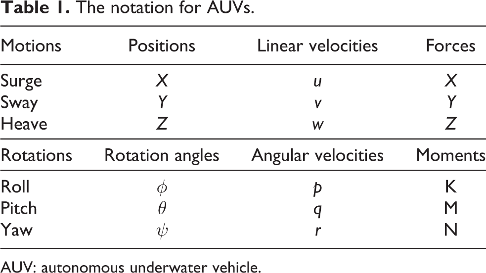
AUV: autonomous underwater vehicle.

In the body-fixed reference frame, a classic 6-DOF model is used to describe the position and orientation of a marine vehicle. ³¹ The translational (surge, sway, and heave) and rotational (roll, pitch, and yaw) equations of the 6-DOF model are written as follows

$\begin{array}{l}m\left[\dot{u}-vr+wq-x_G\left(q^2+r^2\right)+y_G\left(pq-\dot{r}\right)+\right.z_G\hfill \\ \left.\left(pr+\dot{q}\right)\right]=X\hfill \\ m\left[\dot{v}-wp+ur-y_G\left(r^2+p^2\right)+z_G\left(qr-\dot{p}\right)+x_G\right.\hfill \\ \left.\left(qp+\dot{r}\right)\right]=Y\hfill \\ m\left[\dot{w}-uq+vp-z_G\left(p^2+q^2\right)+x_G\left(rp-\dot{q}\right)+y_G\right.\hfill \\ \left.\left(rq+\dot{p}\right)\right]=Z\hfill \\ I_x\dot{p}+\left(I_x-I_y\right)qr-I_{xz}\left(\dot{r}+pq\right)+I_{yz}\left(r^2-q^2\right)+I_{xy}\hfill \\ \left(pr-\dot{q}\right)+m{y}_G\left(\dot{w}+pv-qu\right)-m{z}_G\left(\dot{v}+ru-pw\right)=K\hfill \\ I_y\dot{q}+\left(I_x-I_z\right)rp-I_{xy}\left(\dot{p}+qr\right)+I_{xz}\left(p^2-r^2\right)+I_{yz}\hfill \\ \left(pq-\dot{r}\right)+m{z}_G\left(\dot{u}+qw-vr\right)-m{x}_G\left(\dot{w}+pv-qu\right)=M\hfill \\ I_z\dot{r}+\left(I_y-I_x\right)pq-I_{yz}\left(\dot{q}+pr\right)+I_{xy}\left(q^2-p^2\right)+I_{xz}\hfill \\ \left(qr-\dot{p}\right)+m{x}_G\left(\dot{v}+ru-pw\right)-m{y}_G\left(\dot{u}+qw-rv\right)=N\hfill \end{array}$

1

where m is the mass of the AUV (kg), u,v,w are the velocities of surge, sway, and heave (m/s), p,q,r are the angular velocities of roll, pitch, and yaw (rad/s), $x_G,y_G,z_G$ are the center of gravity (m), $I_x,I_y,I_z$ are the mass moments of inertia (N m²), $I_{xy},I_{xz},I_{yz}$ are the moments of inertia (N m²), X,Y,Z are the external forces (N), and K,M,N are the external moments (N m).

In equation (1), there are six equations, and each equation describes the relationship between external force and system states. In addition, each state is relative to the other five states, and it is difficult to solve this problem in SI. To reduce the model complexity, it is necessary to simplify equation(1) as follows:

Assuming that the hull is symmetry and the mass distribution is symmetrical to the plane;

Assuming that the static force and buoyancy are balanced;

Omitting the coupling of vertical plane motion to horizontal motion and ignoring some of the secondary hydrodynamic coefficients.

According to the assumptions, the forces and moments X,Y,Z,K,M,N, which are the results of combined effects of the various external forces, can be expressed as

$\begin{array}{ll}X=\hfill & \frac{\rho }{2}{l}^4\left(X_{qq}{q}^2+X_{rr}{r}^2\right)+\frac{\rho }{2}{l}^3\left(X_{\dot{u}}\dot{u}+X_{wq}wq\right)\hfill \\ \hfill & +\frac{\rho }{2}{l}^2{u}^2\left(X_{{\delta }_r{\delta }_r}{\delta }_r^2+X_{{\delta }_s{\delta }_s}{\delta }_s^2+X_{{\delta }_b{\delta }_b}{\delta }_b^2\right)\hfill \\ \hfill & +\frac{\rho }{2}{l}^2\left(X_{uu}{u}^2+X_{ww}{w}^2\right)\hfill \end{array}$

2

$\begin{array}{ll}Y=\hfill & \frac{\rho }{2}{l}^4\left(Y_{\dot{r}}\dot{r}+Y_{\dot{p}}\dot{p}+Y_{p\left|p\right|}p\left|p\right|+Y_{pq}pq\right)\hfill \\ \hfill & +\frac{\rho }{2}{l}^3\left(Y_{\dot{v}}\dot{v}+Y_{wp}wp+Y_{r}ur+Y_{p}up\right)\hfill \\ \hfill & +\frac{\rho }{2}{l}^3\left(Y_{v}uv+Y_{v\left|v\right|}v\left|{\left(v^2+w^2\right)}^{\frac{1}{2}}\right|\right)\hfill \\ \hfill & +\frac{\rho }{2}{l}^2{Y}_{{\delta }_r}{u}^2{\delta }_r+\frac{\rho }{2}{l}^2(\eta -1)Y_{{\delta }_r\eta }{\delta }_r{u}^2\hfill \end{array}$

3

$\begin{array}{ll}Z=\hfill & \frac{\rho }{2}{l}^4\left(Z_{\dot{q}}\dot{q}+Z_{rr}{r}^2+Z_{rp}rp\right)\hfill \\ \hfill & +\frac{\rho }{2}{l}^3\left(Z_{\dot{w}}\dot{w}+Z_{q}uq\right)+\frac{\rho }{2}{l}^2\left(Z_{*}{u}^2+Z_{w}uw\right)\hfill \end{array}$

4

$\begin{array}{ll}K=\hfill & \frac{\rho }{2}{l}^5\left(K_{\dot{p}}\dot{p}+K_{\dot{r}}\dot{r}+K_{qr}qr+K_{p\left|\text{p}\right|}p\left|p\right|\right)\hfill \\ \hfill & +\frac{\rho }{2}{l}^4\left(K_{p}up+K_{r}ur+K_{wp}wp\right)\hfill \\ \hfill & +\frac{\rho }{2}{l}^3\left(K_{v}uv+K_{{\delta }_r}{u}^2{\delta }_r\right)\hfill \\ \hfill & -\left(z_{G}W-z_{B}B\right)\text{cos}\theta \text{sin}\phi \hfill \end{array}$

5

$\begin{array}{ll}M=\hfill & \frac{\rho }{2}{l}^5\left(M_{\dot{q}}\dot{q}+M_{q\left|q\right|}q\left|q\right|+M_{rr}{r}^2\right)\hfill \\ \hfill & +\frac{\rho }{2}{l}^3\left(M_{w}uw+M_{{\delta }_s}{u}^2{\delta }_s+M_{{\delta }_b}{u}^2\delta \right)\hfill \\ \hfill & +\frac{\rho }{2}{l}^4\left(M_{\dot{w}}\dot{w}+M_{q}uq\right)-\left(z_{G}W-z_{B}B\right)\text{sin}\theta \hfill \end{array}$

6

$\begin{array}{ll}N=\hfill & \frac{\rho }{2}{l}^5\left(N_{\dot{r}}\dot{r}+N_{\dot{p}}\dot{p}+N_{pq}pq+N_{r\left|r\right|}r\left|r\right|\right)\hfill \\ \hfill & +\frac{\rho }{2}{l}^4\left(N_{\dot{v}}\dot{v}+N_{r}ur+N_{p}up\right)\hfill \\ \hfill & +\frac{\rho }{2}{l}^3\left(N_{v}uv+N_{vw}vw+N_{{\delta }_r}{u}^2{\delta }_r\right)\hfill \\ \hfill & +\frac{\rho }{2}{l}^3\left(\eta -1\right)N_{{\delta }_r\eta }{\delta }_r{u}^2\hfill \end{array}$

7

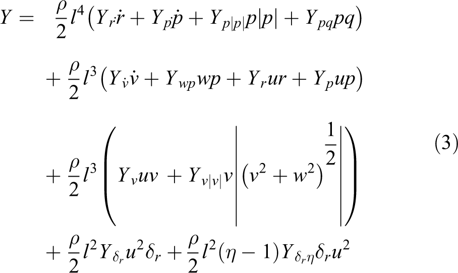
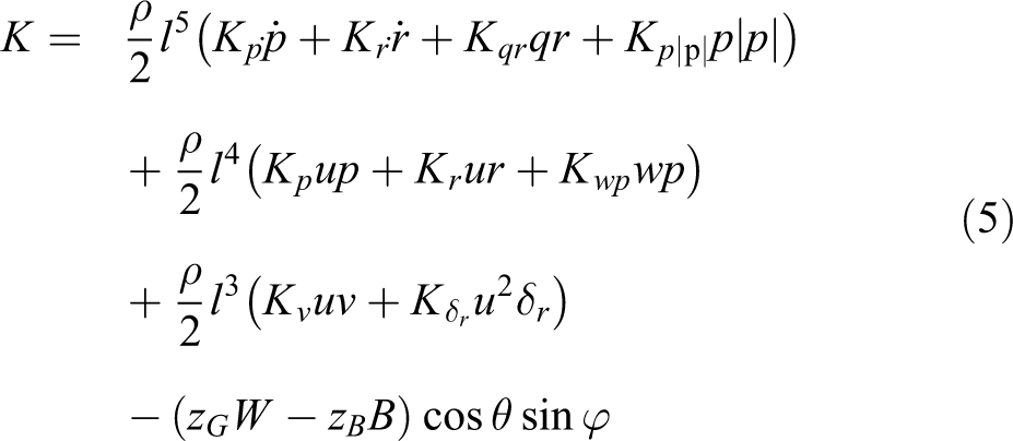
where ρ is the density of liquid around the AUV (kg/m³), l is the length of the AUV (m), $x_B,y_B,z_B$ are the center of buoyancy (N), W is the weight of the AUV (N), B is the buoyancy of the AUV (N), $X_{qq}$ and similar others in equation, are viscous hydrodynamic coefficients. There are totally 56 parameters to be identified, as listed in Table 2. ¹⁸

Table 2.

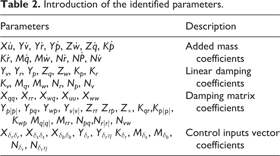
Introduction of the identified parameters.

Parameters	Description
$X_{\dot{u}}$ , $Y_{\dot{v}}$ , $Y_{\dot{r}}$ , $Y_{\dot{p}}$ , $Z_{\dot{w}}$ , $Z_{\dot{q}}$ , $K_{\dot{p}}$ $K_{\dot{r}}$ , $M_{\dot{q}}$ , $M_{\dot{w}}$ , $N_{\dot{r}}$ , $N_{\dot{P}}$ , $N_{\dot{v}}$	Added mass coefficients
Yv , Yr , Yp , Zq , Zw , Kp , Kr Kv , Mq , Mw , Nr , Np , Nv	Linear damping coefficients
$X_{qq}$ , $X_{rr}$ , $X_{wq}$ , $X_{uu}$ , $X_{ww}$ $Y_{p\left|p\right|}$ , $Y_{pq}$ , $Y_{wp}$ , $Y_{v\left|v\right|}$ , $Z_{rr}$ $Z_{rp}$ , $Z_{*}$ , $K_{qr}$ , $K_{p\left|\text{p}\right|}$ , $K_{wp}$ $M_{q\left|q\right|}$ , $M_{rr}$ , $N_{pq}$ , $N_{r\left|r\right|}$ , $N_{vw}$	Damping matrix coefficients
$X_{{\delta }_r{\delta }_r}$ , $X_{{\delta }_s{\delta }_s}$ , $X_{{\delta }_b{\delta }_b}$ , $Y_{{\delta }_r}$ , $Y_{{\delta }_r\eta }$ $K_{{\delta }_r}$ , $M_{{\delta }_s}$ , $M_{{\delta }_b}$ , $N_{{\delta }_r}$ , $N_{{\delta }_r\eta }$	Control inputs vector coefficients

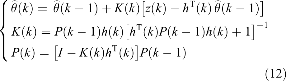
Model identification with MILS

MILS algorithm

The linear time-invariant system is described as follows

$z\left(k\right)=h^{\text{T}}\left(k\right)\theta +e\left(k\right)$

8

where $z\left(k\right)\in R$ is the system output, $h\left(k\right)\in R^n$ is the information vector composed of input and output data, $e\left(k\right)\in R$ is the random noise with zero mean, and $\theta \in R^n$ is the parameter vector to be identified. According to the LS identification theory, ³² the quadratic cost function is

$\begin{array}{c}J\left(\theta \right)={\displaystyle \sum _{k=1}^L}\left[e{(k)}^2\right]={\displaystyle \sum _{k=1}^L}{\left[z(k)-h^{\text{T}}\left(k\right)\theta \right]}^2\\ \\ ={\left(z_L-H_L\theta \right)}^{\text{T}}\left(z_L-H_L\theta \right)\end{array}$

9

Assuming that the parameter vector $\stackrel{⌢}{\theta }\left(k\right)$ makes that $J\left(\theta \right){|}_{\stackrel{⌢}{\theta }\left(k\right)}=\text{min}$ . Since $J\left(\theta \right)$ is quadratic in θ, we can easily get the $\stackrel{⌢}{\theta }\left(k\right)$ by setting the derivative to zero

${\frac{\partial J\left(\theta \right)}{\partial \theta }}_{\stackrel{⌢}{\theta }\left(k\right)}=\frac{\partial }{\partial \theta }{\left(z_L-H_L\theta \right)}^{\text{T}}\left(z_L-H_L\theta \right)=0$

10

which gives

$\stackrel{⌢}{\theta }\left(k\right)={\left(H_L^{\text{T}}{H}_L\right)}^{-1}{H}_L^{\text{T}}{z}_L$

11

The method to obtain $\stackrel{⌢}{\theta }\left(k\right)$ by using equation (11) is the LS method. On the basis of the LS, it is easy to derive the RLS algorithm. When measurements are available, the parameters $\stackrel{⌢}{\theta }\left(k\right)$ are computed at each time k by adding a correction term to the parameters $\stackrel{⌢}{\theta }\left(k-1\right)$ of the previous time. The RLS can be written as follows

$\left\{\begin{array}{l}\stackrel{⌢}{\theta }\left(k\right)=\stackrel{⌢}{\theta }\left(k-1\right)+K\left(k\right)\left[z\left(k\right)-h^{\text{T}}\left(k\right)\stackrel{⌢}{\theta }\left(k-1\right)\right]\hfill \\ K\left(k\right)=P\left(k-1\right)h\left(k\right){\left[h^{\text{T}}\left(k\right)P\left(k-1\right)h\left(k\right)+1\right]}^{-1}\hfill \\ P\left(k\right)=\left[I-K\left(k\right)h^{\text{T}}\left(k\right)\right]P\left(k-1\right)\hfill \end{array}\right.$

12

where $P\left(k\right)$ is the covariance matrix, its dimension depends on the number of identification parameters. The initial value $\stackrel{⌢}{\theta }\left(0\right)$ is a fully small real vector. The initial value $P\left(0\right)=\gamma I\in R^{n\times n}$ is a fully large real unit matrix.

In the RLS, the error $e\left(k\right)=z\left(k\right)-h^{\text{T}}\left(k\right)\theta \left(k-1\right)$ is regarded as the single innovation scalar. To make full use of the past information data, considering to expand the single innovation scalar $e\left(k\right)\in R$ to the multi-innovation vector $E\left(l,k\right)\in R^l$ with length l

$E\left(l,k\right)=\left[\begin{array}{c}e\left(k\right)\\ e\left(k-1\right)\\ ⋮\\ e\left(k-l+1\right)\end{array}\right]\in R^l$

13

where the positive integer l denotes the innovation length. As for the single innovation scalar $e\left(k-i\right)$

$e\left(k-i\right)=z\left(k-i\right)-h^{\text{T}}\left(k-i\right)\stackrel{⌢}{\theta }\left(k-i-1\right)$

14

In general, it is easy to prove that the parameter $\stackrel{⌢}{\theta }\left(k-1\right)$ at the time $k-1$ is closer to θ than $\stackrel{⌢}{\theta }\left(k-i\right)$ at the time $k-i\left(i=2,3,\cdots ,l-1\right)$ . Thus, it would be more reasonable for the multi-innovation vector to be

$E\left(l,k\right)=\left[\begin{array}{c}z\left(k\right)-h^{\text{T}}\left(k\right)\stackrel{⌢}{\theta }\left(k-1\right)\\ z\left(k-1\right)-h^{\text{T}}\left(k-1\right)\stackrel{⌢}{\theta }\left(k-1\right)\\ ⋮\\ z\left(k-l+1\right)-h^{\text{T}}\left(k-l+1\right)\stackrel{⌢}{\theta }\left(k-1\right)\end{array}\right]$

15

According to the multi-innovation identification theory, ³³ the input matrix $h\left(l,k\right)$ and the output matrix $z\left(l,k\right)$ are similarly extended as

$\begin{array}{l}h\left(l,k\right)=\left[h\left(k\right),h\left(k-1\right),\cdots ,h\left(k-l+1\right)\right]\hfill \\ \hfill \\ z\left(l,k\right)=\left[z\left(k\right),z\left(k-1\right),\cdots ,z\left(k-l+1\right)\right]\hfill \end{array}$

16

After replacing the innovation, input matrix, and output matrix, the multi-innovation vector can be easily expressed as

$E\left(l,k\right)=z\left(l,k\right)-h^{\text{T}}\left(l,k\right)\stackrel{⌢}{\theta }\left(k-1\right)$

17

Obviously, when the innovation length l is 1, $E\left(1,k\right)=e\left(k\right)$ , $h\left(1,k\right)=h\left(k\right)$ , and $z\left(1,k\right)=z\left(k\right)$ . So, similarly, as the RLS, the MILS with the innovation length l is written as

$\left\{\begin{array}{l}\stackrel{⌢}{\theta }\left(k\right)=\stackrel{⌢}{\theta }\left(k-1\right)+K\left(k\right)\left[z\left(l,k\right)-h^{\text{T}}\left(l,k\right)\stackrel{⌢}{\theta }\left(k-1\right)\right]\hfill \\ K\left(k\right)=P\left(k-1\right)h\left(l,k\right){\left[h^{\text{T}}\left(l,k\right)P\left(k-1\right)h\left(l,k\right)+1\right]}^{-1}\hfill \\ P\left(k\right)=\left[I-K\left(k\right)h^{\text{T}}\left(l,k\right)\right]P\left(k-1\right)\hfill \\ h\left(l,k\right)=\left[h\left(k\right),h\left(k-1\right),\cdots ,h\left(k-l+1\right)\right]\hfill \\ z\left(l,k\right)={\left[z\left(k\right),z\left(k-1\right),\cdots ,z\left(k-l+1\right)\right]}^{\text{T}}\hfill \end{array}\right.$

18

Clearly, when $l=1$ , the MILS reduces to the RLS. Since the MILS repeatedly uses the current time data and past multiple time data $\left\{z\left(k-i\right),h\left(k-i\right):i=0,1,\cdots ,l-1\right\}$ , it shows better performance in parameter identification in comparison with the RLS.

Identification of 6-DOF equations of motion

In this section, all of the six equations will be identified to obtain the hydrodynamic coefficients. According to the MILS, the 6-DOF dynamic equations can be simply organized as

$\left[\begin{array}{c}\dot{u}\\ \dot{v}\\ \dot{w}\\ \dot{p}\\ \dot{q}\\ \dot{r}\end{array}\right]=\left[\begin{array}{cccccc}{h}_1^{\text{T}}& h_2^{\text{T}}& h_3^{\text{T}}& h_4^{\text{T}}& h_5^{\text{T}}& h_6^{\text{T}}\end{array}\right]\left[\begin{array}{c}{\theta }_1\\ {\theta }_2\\ {\theta }_3\\ {\theta }_4\\ {\theta }_5\\ {\theta }_6\end{array}\right]$

19

Take the surge motion equation $\dot{u}\left(k\right)=h_1^{\text{T}}\left(k\right){\theta }_1$ as an example to estimate the hydrodynamic coefficients. Since it is difficult to assign an initial value to the parameter ${\theta }_1$ in the recursive process, we usually make that ${\theta }_1\left(0\right)=0$ . It is equivalent to using the first recursive identification result of the parameter as the initial value

$\dot{u}=h_1^{\text{T}}{\theta }_1={\left[\begin{array}{c}{q}^2\\ r^2\\ wq\\ u^2\\ w^2\\ u^2{\delta }_r{}^2\\ u^2{\delta }_b{}^2\\ u^2{\delta }_s{}^2\\ mvr-wq-z_G\left(pr+\dot{q}\right)+X_T\end{array}\right]}^{\text{T}}{\theta }_1$

20

$\begin{array}{r}\hfill {\theta }_1=\left[\frac{0.5\rho l^4{X}_{qq}}{m-0.5\rho l^3{X}_{\dot{u}}},\frac{0.5\rho l^4{X}_{rr}}{m-0.5\rho l^3{X}_{\dot{u}}},\frac{0.5\rho l^3{X}_{wq}}{m-0.5\rho l^3{X}_{\dot{u}}},\right.\\ \hfill \frac{0.5\rho l^2{X}_{uu}}{m-0.5\rho l^3{X}_{\dot{u}}},\frac{0.5\rho l^4{X}_{ww}}{m-0.5\rho l^3{X}_{\dot{u}}},\frac{0.5\rho l^4{X}_{{\delta }_r{\delta }_r}}{m-0.5\rho l^3{X}_{\dot{u}}},\\ \hfill {\left.\frac{0.5\rho l^4{X}_{{\delta }_b{\delta }_b}}{m-0.5\rho l^3{X}_{\dot{u}}},\frac{0.5\rho l^4{X}_{{\delta }_s{\delta }_s}}{m-0.5\rho l^3{X}_{\dot{u}}},\frac{1}{m-0.5\rho l^3{X}_{\dot{u}}}\right]}^{\text{T}}\end{array}$

21

where X_T denotes the constant thrust produced by the stern propeller. Then, taking N sample data to obtain the following matrix equation

$\underset{z\left(k\right)}{\underbrace{\dot{U}(N)}}=\underset{h^{\text{T}}\left(k\right)}{\underbrace{H_1^{\text{T}}(N)}}\underset{\theta }{\underbrace{{\theta }_1}}$

22

where

$\dot{U}(N)=\left[\begin{array}{c}\dot{u}(1)\\ \dot{u}(2)\\ \dot{u}(3)\\ ⋮\\ \dot{u}(N)\end{array}\right]$

23

$H_1^{\text{T}}(N)=\left[\begin{array}{ccc}{q}^2(1)& \cdots & mv(1)w(1)-\cdots +X_T(1)\\ q^2(2)& \cdots & mv(2)w(2)-\cdots +X_T(2)\\ q^2(3)& \cdots & mv(3)w(3)-\cdots +X_T(3)\\ ⋮& ⋮& ⋮\\ q^2(N)& \cdots & mv(N)w(N)-\cdots +X_T(N)\end{array}\right]$

24

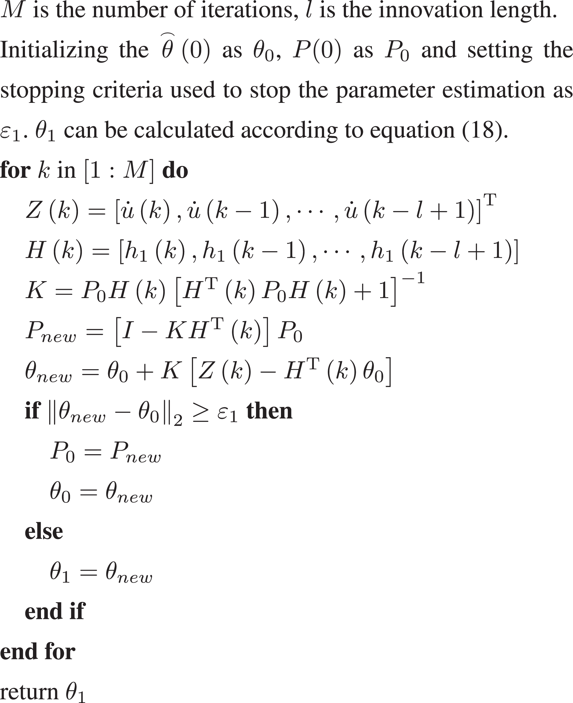
In this way, the identification problem is turned into the linear fitting problem and the identified model is only in relation with the system input and output. The procedure of surge motion equation parameter identification method based on MILS is shown in Algorithm 1. According to the value of ${\theta }_1$ estimated by the MILS, we can easily obtain the hydrodynamic coefficients $X_{\dot{u}},X_{qq},X_{rr},X_{wq},X_{uu},X_{ww},X_{{\delta }_r{\delta }_r},X_{{\delta }_b{\delta }_b},X_{{\delta }_s{\delta }_s}$ in turn. The same procedure can be applied to other five equations to get all the parameters.

Algorithm 1.

The surge motion equation identified by MILS.

Validation

Model validation is an indispensable part of the identification process. In this section, we assume that the identified model accurately describes the motion characteristics of the AUV. In addition, the computer used for simulation in this part is described as follows: Lenovo Laptop/Processor: Intel Core i5-4200 M CPU 2.50 GHz/Installed Memory (RAM): 8.00 GB/Operating System: win7 ultimate 64-bit.

Validation flow

For the convincing verification, we divide the identification data obtained from different filed experiments into two data sets. One is the training data that are used to identify hydrodynamic coefficients and the other one is the validation data that are the fresh data used to verify the accuracy of the model. The validation procedure is shown in Figure 2, and the specific steps are described as follows:

Figure 2.

The validation flow.

• Ensuring that all the onboard sensor work normally, then several field experiments have been run with the system input shown in Figure 3 to collect the training data and validation data;

• Using the training data to identify the parameters based on the LS, RLS, and MILS;

• Using the different identified models and the validation data for comparisons.

Figure 3.

The system input of (a) propeller thrust and (b to d) rudder angles.

In addition, the sampling interval in the field experiment is set as 0.1 s, and the simulations are conducted by MATLAB 2016b software. According to the performances of the MILS, RLS, and LS, this article analyzes the convergence rate and the identification accuracy systematically.

Identification convergence analysis

At first, different algorithms identify the parameters of the AUV model with the same training data. The identification results based on the LS, RLS, and MILS with different innovation lengths $\left(l=3,5\right)$ are summarized in Table 3. According to these parameters, we can easily obtain the corresponding identified models. Figure 4 shows the curves of some partial important hydrodynamic coefficients during the identification $\left(X_{{\delta }_s{\delta }_s},Y_{\dot{v}},Z_{\dot{w}},K_{\dot{p}},M_{q\left|q\right|},N_r\right)$ . It is worth noting that as a one-time completion algorithm, LS is not fit for online identification. In addition, the identification needs much more time while the parameter number is large.

Table 3.

The identification results of all the hydrodynamic coefficients.

Method	LS	RLS $\left(l=1\right)$	MILS $\left(l=3\right)$	MILS $\left(l=5\right)$	Method	LS	RLS $\left(l=1\right)$	MILS $\left(l=3\right)$	MILS $\left(l=5\right)$
$X_{\dot{u}}$	−6.81 × 10−4	−4.98 × 10−4	−4.83 × 10−4	−4.6 × 10−4	$K_{\dot{p}}$	−1.1 × 10−4	−1.3 × 10−4	−9.4 × 10−5	−7 × 10−5
$X_{qq}$	−2.32 × 10−3	−2.01 × 10−3	−1.626 × 10−3	−1.443 × 10−3	$K_{\dot{r}}$	−3.5 × 10−4	−3.2 × 10−4	−2.4 × 10−4	−2.8 × 10−4
$X_{rr}$	2.03 × 10−3	1.88 × 10−3	2.17 × 10−3	2.53 × 10−3	$K_{qr}$	7.4 × 10−4	6.7 × 10−4	4.6 × 10−4	3.1 × 10−4
$X_{wq}$	−0.0196	−0.0174	−0.0141	−0.0132	$K_{p\left|\text{p}\right|}$	−8.6 × 10−4	−8.3 × 10−4	−4.83 × 10−4	−3.3 × 10−4
$X_{uu}$	−1.32 × 10−3	−1.46 × 10−3	−1.23 × 10−3	−1.1 × 10−3	Kp	−7.2 × 10−4	−7.9 × 10−4	−6.2 × 10−4	−5.4 × 10−4
$X_{ww}$	9.06 × 10−3	6.83 × 10−3	7.62 × 10−3	7.75 × 10−3	Kr	2.2 × 10−4	2.6 × 10−4	3.4 × 10−4	4.5 × 10−4
$X_{{\delta }_r{\delta }_r}$	−4.93 × 10−3	−4.81 × 10−3	−4.2 × 10−3	−3.9 × 10−3	$K_{wp}$	−8.9 × 10−4	−7.1 × 10−4	−3.6 × 10−4	−2.9 × 10−4
$X_{{\delta }_s{\delta }_s}$	−1.94 × 10−3	−8.8 × 10−4	−9.7 × 10−4	−1.19 × 10−3	Kv	−7.53 × 10−3	−7.06 × 10−3	−3.61 × 10−3	−2.87 × 10−3
$X_{{\delta }_b{\delta }_b}$	−3.62 × 10−3	−3.58 × 10−3	−3.21 × 10−3	−2.99 × 10−3	$K_{{\delta }_r}$	−8.4 × 10−5	−2.5 × 10−5	−3.9 × 10−5	−5 × 10−5
$Y_{\dot{v}}$	−0.0593	−0.0583	−0.0579	−0.0613	$M_{\dot{q}}$	−7.6 × 10−4	−8.8 × 10−4	−9.3 × 10−4	−9.8 × 10−4
$Y_{\dot{r}}$	−1.81 × 10−3	−1.84 × 10−3	−1.95 × 10−3	−2.26 × 10−3	$M_{q\left|q\right|}$	−4.83 × 10−3	−4.65 × 10−3	−3.53 × 10−3	−3.03 × 10−3
$Y_{\dot{p}}$	−8.32 × 10−4	−8.21 × 10−4	−7.9 × 10−4	−6 × 10−4	$M_{rr}$	−2.91 × 10−3	−2.88 × 10−3	−2.23 × 10−3	−1.14 × 10−3
$Y_{p\left|p\right|}$	5.22 × 10−3	5.15 × 10−3	4.88 × 10−3	4.65 × 10−3	$M_{\dot{w}}$	−1.92 × 10−3	−1.86 × 10−3	−1.43 × 10−3	−1.38 × 10−3
$Y_{pq}$	8.42 × 10−3	5.81 × 10−3	6.8 × 10−3	7.3 × 10−3	Mq	−5.14 × 10−3	−4.74 × 10−3	−4.12 × 10−3	−3.89 × 10−3
$Y_{wp}$	−0.0094	−0.0052	−0.0162	0.0144	Mw	1.47 × 10−4	2.96 × 10−4	3.83 × 10−4	4.78 × 10−3
Yv	−0.0527	−0.0427	−0622	−0.0654	$M_{{\delta }_s}$	−0.025	−0.033	−0.019	−0.023
$Y_{v\left|v\right|}$	−0.113	−0.081	−0.0271	−0.029	$M_{{\delta }_b}$	7.24 × 10−3	8.98 × 10−3	9.12 × 10−3	9.4 × 10−3
Yr	−4.85 × 10−3	−4.81 × 10−3	9.7 × 10−3	2.3 × 10−4	$N_{\dot{r}}$	−3.92 × 10−3	−3.74 × 10−3	−3.51 × 10−3	−4.82 × 10−3
Yp	−1.2 × 10−3	−1.5 × 10−3	−3.1 × 10−3	−4.5 × 10−3	$N_{\dot{p}}$	−4.9 × 10−5	−3.5 × 10−5	−3.3 × 10−5	−3.1 × 10−5
$Y_{{\delta }_r}$	−6.4 × 10−3	−5.9 × 10−3	−8.7 × 10−4	−8.3 × 10−4	$N_{pq}$	−8.5 × 10−4	−6.5 × 10−4	−8.4 × 10−4	−9.1 × 10−4
$Y_{{\delta }_r\eta }$	1.2 × 10−4	3.5 × 10−4	5.2 × 10−4	6.7 × 10−4	$N_{r\left|r\right|}$	2.71 × 10−3	2.25 × 10−3	2.14 × 10−3	2.05 × 10−3
$Z_{\dot{w}}$	−0.0193	−0.0182	−0.0164	−0.0144	$N_{\dot{v}}$	7.1 × 10−4	7.3 × 10−4	5.4 × 10−4	6.8 × 10−4
$Z_{\dot{q}}$	−6 × 10−5	−6 × 10−5	−6 × 10−5	−7 × 10−5	Nr	−4.78 × 10−3	−4.88 × 10−3	−4.96 × 10−3	−4.83 × 10−3
$Z_{rr}$	−5.13 × 10−3	−4.73 × 10−3	−4.25 × 10−3	−3.96 × 10−3	Np	−7.02 × 10−4	−5.12 × 10−4	−4.93 × 10−4	−6.8 × 10−4
$Z_{rp}$	−3.01 × 10−3	−3.81 × 10−3	−2.31 × 10−3	−1.9 × 10−3	Nv	−0.0094	−0.0186	−0.032	−0.029
Zq	−8.36 × 10−3	−7.56 × 10−3	−7.22 × 10−3	−6.99 × 10−3	$N_{vw}$	−0.3408	−0.3324	−0.3227	−0.3172
$Z_{*}$	−6.1 × 10−3	−5.2 × 10−3	−3 × 10−4	−1.18 × 10−3	$N_{{\delta }_r}$	−3.56 × 10−3	−3.34 × 10−3	−2.83 × 10−3	−1.12 × 10−3
Zw	−0.0083	−0.0095	−0.0188	−0.0203	$N_{{\delta }_r\eta }$	−3.1 × 10−5	−2.8 × 10−5	−8.8 × 10−5	−3.42 × 10−4

LS: least square; RLS: recursive least squares; MILS: multi-innovation least squares.

Figure 4.

(a to f) Estimation of partial hydrodynamic coefficients.

In Figure 4, the x-axis indicates the iteration number, and the y-axis indicates the parameter values. The parameter curves show that each parameter eventually converges to a specific value with different convergence rates. Table 4 lists the convergence time of these hydrodynamic coefficients with different identification algorithms. The results show that the following:

Table 4.

The convergence times of the parameters.

Method	RLS $\left(l=1\right)$	MILS $\left(l=3\right)$	MILS $\left(l=5\right)$
$X_{{\delta }_s{\delta }_s}$	157	30	25
$Y_{\dot{v}}$	291	32	18
$Z_{\dot{w}}$	256	19	11
$K_{\dot{p}}$	166	40	30
$M_{q\left|q\right|}$	145	106	53
Nr	289	37	30

RLS: recursive least squares; MILS: multi-innovation least squares.

• The convergence time of MILS is always less than that of the RLS while the innovation length is set to different values.

• The convergence rate of MILS becomes faster when the innovation length is larger. However, the large innovation length also means more complex computation, and then, it is necessary to choose reasonable innovation length.

• Because the convergence of the MILS is faster than RLS, it needs fewer sample data than RLS to identify the system parameter. When the innovation length is larger, the MILS is able to approximate the optimal parameters with small sample data.

Identification accuracy analysis

We use the fourth-order Runge–Kutta ordinary differential equation (ODE) integration algorithm to solve the hydrodynamic equations identified by LS, RLS, and MILS, respectively. In the field of statistics, mean absolute error (MAE) is often used to evaluate the error between actual and predicted values. In this article, we use the MAE to measure the accuracy of the identification. With the same system input, the MAE between the simulated velocity y_i and the actual velocity y_e is

$\text{MAE}=\frac{1}{N}{\displaystyle \sum _{k=1}^N}\left|y_i\left(k\right)-y_e\left(k\right)\right|$

25

Figure 5 shows the actual measurements and the simulated velocities based on different models. Table 5 lists the MAE between actual data and the simulation results. The comparisons are as follows:

Figure 5.

(a to f) Comparison of the identification data and the validation data.

Table 5.

Comparisons of the MAE between the identification velocities and experimental velocities.

Method	LS	RLS $\left(l=1\right)$	MILS $\left(l=3\right)$	MILS $\left(l=5\right)$
u	0.528	0.495	0.355	0.182
v	2.52 × 10−4	1.85 × 10−4	1.24 × 10−4	9.39 × 10−5
w	7.34 × 10−3	6.59 × 10−3	4.27 × 10−3	3.2 × 10−3
p	7.21 × 10−4	7.8 × 10−4	4.95 × 10−4	3.82 × 10−4
q	1.14 × 10−3	8.89 × 10−4	5.34 × 10−4	3.21 × 10−4
r	1.26 × 10−3	1.19 × 10−3	7.23 × 10−4	4.91 × 10−4

LS: least square; RLS: recursive least squares; MILS: multi-innovation least squares; MAE: mean absolute error.

• When $l=3$ and $l=5$ , the MAE results of the MILS are lower than those of the LS and RLS. These performances are consistent with expectations from theoretical analysis.

• When $l=5$ , the MAE of MILS is the lowest among the four models. It means that the identification accuracy of MILS is relative to the innovation length. Although large innovation length improves the identification accuracy of MILS, it also needs complex computation.

The convergence rate and identification accuracy results show that the MILS is more effective to identify the parameters of the AUV model than the LS and RLS.

Conclusions

In this article, we employ the MILS algorithm to identify a simplified 6-DOF AUV model. The simplified model only contains the essential parameters of the nonlinear kinetic model that includes hundreds of hydrodynamic coefficients, so it is useful for engineering applications in practice. The MILS algorithm leverages several past errors to identify the parameters, it not only converges faster than the RLS but also approximates more accurate than the RLS. In addition, the MILS needs fewer sample data to identify the parameter than the LS and RLS. Large innovation length improves the convergence rate and accuracy of the MILS, but it increases the computation load. Different model has a different property, it is necessary to choose reasonable innovation length according to the model characteristic. Future work will focus on the identification algorithm that is used to identify the parameters when the AUV is disturbed by the external environment.