Sage Journals: Discover world-class research

Abstract

In robotics, solving the direct kinematics problem (DKP) for parallel robots is very often more difficult and time consuming than for their serial counterparts. The problem is stated as follows: given the joint variables, the Cartesian variables should be computed, namely the pose of the mobile platform. Most of the time, the DKP requires solving a non-linear system of equations. In addition, given that the system could be non-convex, Newton or Quasi-Newton (Dogleg) based solvers get trapped on local minima. The capacity of such kinds of solvers to find an adequate solution strongly depends on the starting point. A well-known problem is the selection of such a starting point, which requires a priori information about the neighbouring region of the solution. In order to circumvent this issue, this article proposes an efficient method to select and to generate the starting point based on probabilistic learning. Experiments and discussion are presented to show the method performance. The method successfully avoids getting trapped on local minima without the need for human intervention, which increases its robustness when compared with a single Dogleg approach. This proposal can be extended to other structures, to any non-linear system of equations, and of course, to non-linear optimization problems.

Keywords

Hybrid optimizer Probabilistic learning Direct Kinematics Parallel Robots

1. Introduction

In recent years, parallel robots have become an excellent solution for applications where a precise pose (position and orientation) is needed. Such kinds of applications can be found on machining centres and radio telescopes among others. Today, for successful application, the kinematics of these structures requires a robust solution that has a significant role when high accuracy and low computational cost are needed. Depending on a particular configuration, in the simplest cases, the direct kinematics problem of this kind of structure can be solved in closed form. Generally the generalized coordinates cannot be expressed in an analytical manner as functions of the actuated joint coordinates [1]. In these cases, optimization algorithms and non-linear solvers can be used. Due to the characteristics of parallel robots, such as intrinsic closed chains, there is no one to one relationship between controllable variables and degrees of freedom. Thus, each controllable variable affects output degrees of freedom and vice versa. Usually non-linear functions are involved therefore it is not surprising that Newton and Quasi-Newton methods can get trapped on local minima when trying to solve the non-linear system.

One of the best known parallel manipulators is the Stewart platform [2]. Although this structure was first introduced by Gough [3], it is often referred to just as the Stewart platform. Some authors have recognized this paradox and they use the term Gough-Stewart platform. We will refer it as the Stewart platform, without recognizing this fact. It was selected for the case studied here, since this structure can be intended for highly precise applications. In the last two decades, many different aspects of this parallel manipulator have been studied and reported on [4] [5] [6] [7] [8].

There are some configurations that can be referred to as simplified Stewart platforms [9]. They are represented schematically in Fig. 1. Fig. 1 (a) shows the configuration with regular hexagons for the base and mobile platforms. Fig. 1 (b) shows a configuration with similar symmetric hexagons for both platforms. The architecture in Fig. 1 (c), termed SSM (Simplified Symmetric Manipulator), is characterized by the fact that the planar base and platform have an axis of symmetry. The architecture shown in Fig. 1 (e), termed TSSM (Triangular Simplified Symmetric Manipulator), is an SSM manipulator with a triangular platform. The architecture shown in Fig. 1 (d), the MSSM (Minimal Simplified Symmetric Manipulator), is a TSSM with a triangular base. Fig. 1 (f) shows the configuration commonly called the 3-2-1 configuration. In fact, taking into count the location of the joints on the base and mobile platforms, Figs. 1 (a), Fig. 1 (b) and SSM are architectures have a 6-6 configuration, often called general 6-6 Stewart platforms; meanwhile, MSSM is referred to as a 3-3 configuration and TSSM as a 6-3 configuration. The direct kinematics problem of the Stewart platform with a 6-6 configuration has been approached by many researchers in the past. However, research in this area is still continuing, due the lack of an effective solution approach. In fact, no matter what approach for the DKP of a general 6-6 Stewart platform is used, a unique solution is still a challenging problem. Some methodologies have been used: analytical methods, use of redundant sensors, numerical approaches, neural network-based methods, and recently, by using evolutionary algorithms.

Figure 1.

Top view of different configurations for Stewart platforms; (a) configuration with regular hexagons; (b) configuration with similar symmetric hexagons; (c) SSM configuration; (d) MSSM configuration; (e) TSSM configuration; (f) 3-2-1 configuration

In particular, analytical methods have been proposed to address the DKP for a general Stewart platform; their main differences can be explained as: i) by formulating a system of non-linear equations and converting them to higher degree polynomial, after multiple solutions are obtained by finding roots of this polynomial, [10] [11] [12] [13]. These solutions are referred as the assembly modes of the manipulator. ii) The pose parameters can be decoupled, which leads to reduced complexity and computational cost [14]; iii) other analytical methods in the literature include the continuation method [15] [16], elimination methods [17] [18] [19] [20] and interval analysis [10]. However, the DKP is not fully solved just by finding all the possible solutions. For practical purposes, a unique actual pose in the platform workspace is necessary. Moreover, some approaches are not suitable for real-time operation, due their computation time.

Installation of redundant sensors has been proposed to address the DKP [21]. But this approach has practical limitations such as cost and additional measurement errors. On the other hand, the DKP could be solved by using a numerical technique like the Newton-Raphson method [22] [23] [24]. The Newton-Raphson iterative technique has been the most popular method for solving the DKP of parallel robots as in some cases it gives very accurate results. Unfortunately, by using just this technique, there is no guarantee of convergence to the solution and the successful convergence of this method is highly dependent on the starting values for the solution.

Taking the same form, strategies based on neural networks have been proposed [25]. They propose a hybrid method where a neural network achieves the starting values for a Newton-Raphson algorithm. Other approaches have been reported in [26] [27] and[28], and recently [29], for a cable Stewart platform. The main drawback is that training, testing and validation tasks for the neural network demand a lot of information from the robot workspace.

Referring to robotics in general, evolutionary algorithms have begun to be considered for addressing optimization problems. In particular, genetic algorithms have been used from the optimal planning of experiments for the calibration problem of serial robots [30], most recently, for the optimal control of parallel manipulators [31]. In addition, recently a hybrid method based on genetic algorithms has been implemented to address the direct kinematics of the Stewart platform, by finding all real solutions [32]. The approach presented in [33] deals with the synthesis of mechanisms using differential evolution to solve the dimensional and multi-objective problem of planar mechanisms. The main contribution of this work is in the non-linear solver for the non-linear kinematics of the general Stewart platform. We introduce a novel proposal that could be applied to solve difficult non-linear problems which are not convex in general, but have various convex regions in the search space. Derivative free optimizers, such as genetic algorithms, estimation of distribution algorithms and other population-based algorithms, are computationally expensive and must be used when no other more efficient strategy is known. On the other hand, derivative-based algorithms, such as Newton or Cuasi-Newton methods, are quite efficient when the objective function is smooth and convex, but they tend to be trapped in local minima. In this work, a novel approach which takes advantage of both strategies is used, in order to solve the non-linear kinematics of the general Stewart platform with adequate precision and minimum computational effort. Several experiments and discussions are presented to show the method performance. The method successfully avoids getting trapped on a local minimum without the need for human intervention, which increases the robustness of the solver when compared with a single Dogleg approach. The paper is organized as follows: in Section 2, a kinematic model of the general Stewart platform is introduced and corresponding kinematic equations are formulated as an adequate optimization problem in order to implement a hybrid optimizer. In Section 3 a description of the hybrid optimizer implementation is presented. In Section 4, the performance of numerical experiments is shown to validate the proposed method.

2. Problem Formulation: Non-linear Kinematics of the Stewart Platform

A general Stewart platform has been selected for the case studied here. A kinematic model of this platform was formulated by Gosselin in [34]. It is a manipulator with semi-regular hexagons, where the joints are symmetric in pairs. Its kinematic configuration consists of a fixed plate connected through six legs to a mobile platform, Fig. 2. Each leg has a prismatic joint (actuator), a spherical joint at the fixed end and a universal joint at the mobile end. The fixed and mobile platforms can have the same dimensions. In order to improve the mechanism stability, the spherical and universal joints can be located as close as possible. The centre points of the spherical joints are located at radius r_A and the universal joints are located at radius r_B, Fig. 3. A_i is the centre point of each spherical joint (vertex of a hexagon on the base platform), and B_i is the centre point of each universal joint (vertex of a hexagon on the mobile platform), Fig. 3(a) and Fig. 3(b), respectively.

Figure 2.

A scheme for the Stewart platform

Figure 3.

Location of the joints on the base and mobile platforms

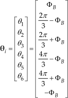
The angular position between the connecting joints is Φ_A at the base platform and Φ_B at the mobile platform. a_i can be referred to as the position vector of each point A with respect to the centre of the base platform and b_i as the position vector of each point B_i with respect to the centre of the mobile platform. Then, they can be written as

a_{i} = [\begin{matrix} r_{A} \cos θ_{i} \\ r_{A} s i n θ_{i} \\ 0 \end{matrix}]

(1)

and

b_{i} = [\begin{matrix} r_{B} \cos η_{i} \\ r_{B} \cos η_{i} \\ 0 \end{matrix}]

(2)

where

θ_{i} = [\begin{matrix} θ_{1} \\ θ_{2} \\ θ_{3} \\ θ_{4} \\ θ_{5} \\ θ_{6} \end{matrix}] = [\begin{matrix} Φ_{B} \\ \frac{2 π}{3} - Φ_{B} \\ \frac{2 π}{3} + Φ_{B} \\ \frac{4 π}{3} - Φ_{B} \\ \frac{4 π}{3} + Φ_{B} \\ - Φ_{B} \end{matrix}]

(3)

and

η_{i} = [\begin{matrix} η_{1} \\ η_{2} \\ η_{3} \\ η_{4} \\ η_{5} \\ η_{6} \end{matrix}] = [\begin{matrix} Φ_{P} \\ \frac{2 π}{3} - Φ_{P} \\ \frac{2 π}{3} + Φ_{P} \\ \frac{4 π}{3} - Φ_{P} \\ \frac{4 π}{3} + Φ_{P} \\ - Φ_{P} \end{matrix}]

(4)

The position vector of the mobile platform is defined as x, (with coordinates x, y, z), and the orientation is found from the rotation matrix R. Thus, the position vector, with respect to the fixed platform of each universal joint (at the mobile platform) can be written as

p_{i} = x + R b_{i} \forall i = 1, 2, …6

(5)

with

R = [\begin{matrix} c α c β & c α s β s δ -s α c δ & c α s β c δ + s α s δ \\ s α c β & s α s β s δ + c α c δ & s α s β c δ - c α s δ \\ - s β & c β s δ & c β c δ \end{matrix}]

(6)

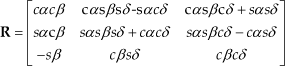
where α, β, δ are the orientation angles of the mobile platform, c, s represent cos() and sin() functions respectively.

Subtracting a_i from both sides of Eq. 5:

p_{i} - a_{i} = x + R b_{i} - a_{i}

(7)

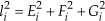
The length l_i of each leg is calculated from the Euclidean norm of Eq. 7 as:

l_{i} = ‖ x + R b_{i} - a_{i} ‖

(8)

In this way, the solution of the inverse kinematic problem can be written as:

l_{i}^{2} = E_{i}^{2} + F_{i}^{2} + G_{i}^{2}

(9)

where

\begin{array}{l} E_{i} = x + R_{11} r_{B} cos η_{i} + R_{12} r_{B} sin η_{i} - r_{A} cos θ_{i} \\ F_{i} = y + R_{21} r_{B} cos η_{i} + R_{22} r_{B} sin η_{i} - r_{A} sin θ_{i} \\ G_{i} = z + R_{31} r_{B} cos η_{i} + R_{32} r_{B} sin η_{i} \end{array}

(10)

recalling that R₁₁, R₁₂, R₂₁… are the components of the matrix R.

In this way, the individual length of each leg is calculated as a function of the position and orientation of the mobile platform. The final position of the mobile platform can be controlled adjusting l_i to a specific length. From Eq. 10, it can be seen that x, y, z and α, β, δ, position and orientation variables depend on the length of the six legs, i.e., the direct kinematic problem consists of finding the pose given the six length legs. The resolution of the direct kinematics is essential for control purposes, on-line simulations and performance analysis, and primordial tasks in real applications. The problem consists of solving the non-linear system of equations in Eq. 10 for the Cartesian coordinates; the system can be completed with additional equations by using the rotation matrix and its invariants. Six residual functions f_i(x˜)=[f₁…f₆] can be formulated as

f_{i} (\tilde{x}) = E_{i}^{2} + F_{i}^{2} + G_{i}^{2} - l_{i}

(11)

Thus, the system of six equations with six unknowns of Eq. 11 can be solved giving a vector x˜=[x,y,z,α,β,δ] which contains the starting values for position and orientation of the mobile platform, and minimizing the function errors as

\min_{\tilde{x}} {‖ f_{i} (\tilde{x}) ‖}

(12)

3. Implementation of the Hybrid Optimizer

In order to minimize Eq. 12 an optimizer is needed. A widely used, effective and efficient optimizer is the Dogleg [35]. Its process is described in Algorithm 1, it is a minimization/maximization method from the family of the trust-region algorithms, which combines the so-called Cauchy and Newton directions (a direction based on the gradient and another based on second derivatives information, respectively). Nevertheless, the Dogleg produces impressive results when the function to minimize is convex, however, it can be trapped on a local minimum if non-convexity and/or many local minima are present.

As a consequence, this method requires an adequate starting point to converge to the global minimum.

Thus, if the user does not have a priori information about the global minimum position, there is no certainty about finding the actual global minimum. To circumvent this issue, we propose using an Estimation of Distribution Algorithm (EDA) [36]. EDAs are powerful evolutionary optimizers which can avoid local minima and do not need derivatives. Nevertheless, EDAs have been proposed as an extension of Genetic Algorithms (GAs) as it has been proven that EDAs are more effective than GAs when the correlation among variables is an important factor in the optimization process.

Algorithm 1

Dogleg

1: Given

\bar{Δ} > 0, Δ_{0} \in (0, \bar{Δ}) and ρ \in (0, \frac{1}{4}]

2: Fork=1,2,… do 3: Obtain p˜(τ) 4: Evaluate ρ_k 5: If ρ_k < ¼ then 6:

Δ_{k + 1} = \frac{1}{4} ‖ {\tilde{p}}_{k} (τ) ‖

7: else 8: If

ρ_{k} > \frac{3}{4} and ‖ {\tilde{p}}_{k} (τ) ‖ = Δ_{k} then

Δ_{k + 1} = min (2 Δ_{k}, \bar{Δ})

10: else 11: Δ_k+1=Δ_k 12: end if 13: end if 14: If ρ_k> η then 15: x_k₊₁=x_k+p˜_p˜(τ) 16: else 17: x_k₊₁=x_k 18: end if 19: end fo

The main subject of this proposal is the parameter optimization of a mechanical system. Considering that each one of the mechanical parts is related one another, the parameters are strongly correlated, thus, an EDA which considers variable dependencies can be an adequate strategy to tackle this problem. Then, the hybrid optimizer is built as follows: an EDA-based multivariate Gaussian model is used to generate starting points for the Dogleg method, thus, we expect to improve the starting points for the Dogleg method through the generations of the EDA. Even though there is no guarantee of finding the global optimum, our experiments show that the hybrid optimizer delivers the global optimum in 100% of the cases. The general description of the EDA method is shown in Algorithm 2, in step 4, the objective function evaluation refers to applying the Dogleg using each point in the population as a starting point, then, the smaller the norm of the function in Eq. 12, the better the individual (starting point) is.

The selection method in step 5 refers to the truncation of 50% of the population with the worst function values. The re-computation step in 6 means the estimation of the mean and covariance matrix of a multivariate Gaussian model by using the remaining individuals after truncation. The initial probability model is a uniform distribution, assuming that initially we do not have information about the optimum location, and such information is inferred through the iterations.

Algorithm 2

EDA implemented with Dogleg algorithm

1: t=0 2:Initialize a probability model p(x,t) (search distribution) 3: Generate a population X from p(x,t) 4: Evaluate X in the objective function (by using the Dogleg) 5: S_t← selection (X_t) 6: Recompute p(x,t+1), such that p(x,t +1) ≈ p(S_t) 7: t=t +1 8: If the stop criterion is not reached go to 3.

4. Experiments and Results

Our proposal has as its main objective to reduce the human intervention dependency of the optimizer, by sampling random points as starting points of the Dogleg algorithm. Thus, the local Dogleg optimizer is turned into a hybrid global optimizer which uses an EDA and the Dogleg. The EDA's main function is to learn about and use the best regions in the search space to sample random points in order to reduce the computational cost. Notice that we can draw random points using a uniform distribution, but using this strategy means that there is no preference for any region in the search space and the algorithm does not learn how to draw better points. On the other hand, we expect that the EDA is capable of training the parameters of the multivariate Gaussian distribution to sample intensively the most promising regions. We expect that our proposal infers the most promising regions and obtains the information needed to estimate an adequate approximation to the optimum faster than the uniform distribution.

4.1 Contrasting EDA-based Gaussian and Uniform Distributions

We contrast our proposal with another global optimizer which uses a uniform distribution to draw starting points. For our experiments we use 20 well-distributed points in the platform workspace, i.e., we want to solve the direct kinematics problem for 20 different postures of the parallel manipulator. We run the hybrid algorithm and the algorithm based on the uniform distribution100 times, and we statistically test if one of them is better (perform less Dogleg-minimizations) than the other. In other words, let us define x* as a closed approximation to the global optimum (the norm in Eq. 12 is less or equal to 1e-6). To find x, different random starting points are used and the corresponding six lengths are computed by solving the inverse kinematics (Eq. 8). Then, with these lengths a Dogleg-minimization process is run for each one, until the algorithm converges to an optimum approximation with the desired precision.

To draw the random starting points, we can utilize two different approaches:

by using a uniform distribution and

by using the EDA based on a multivariate Gaussian distribution, shown in Algorithm 2.

We contrast these two approaches according to the number of Dogleg-minimizations they need to reach the desired optimum approximation.

Let u be the mean of the number Dogleg-minimizations performed when the random starting points are uniformly generated and μ_n the mean of the Dogleg-minimizations performed by the EDA proposed in Algorithm 2. Then we perform a two hypothesis test:

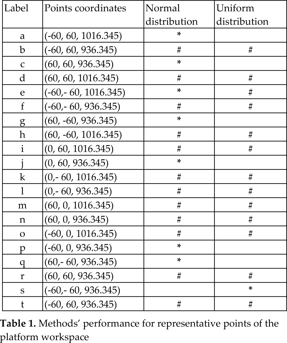
a) We test if μ_u < μ_n (as alternative hypothesis) and b) μ_u > μ_n (as alternative hypothesis). Notice that even though the tests are related, rejecting the first test does not mean accepting the second. In order to avoid assuming a given distribution for the test, we use the Bootstrap methodology [37]. The 20 points tested are labelled as presented in Table 1. We used arbitrary values for orientation parameters in each experiment. The last two columns represent the obtained results. When the decision is better made using a specific distribution (normal or uniform), the corresponding point is labelled with an asterisk (*). In the other case, when no decision can be made given the obtained values, both columns are marked with a hash symbol (#). From Table 1 it can be seen that in seven points out of 20, the normal distribution was better, whereas the uniform distribution was better in just one point. We can assume that the EDA based on a multivariate Gaussian distribution learns about some local minimizations to speed up the optimum estimation with the desired precision and even though the method does not speed up the process in all cases, we can say that (according to statistical evidence) our method will never perform worse than simply drawing uniform starting points.

Table 1.

Methods' performance for representative points of the platform workspace

Label	Points coordinates	Normal distribution	Uniform distribution
a	(−60, 60, 1016.345)	*
b	(−60, 60, 936.345)	#	#
c	(60, 60, 936.345)	*
d	(60, 60, 1016.345)	#	#
e	(−60, −60, 1016.345)	*	#
f	(−60, −60, 936.345)	#	#
g	(60, −60, 936.345)	*
h	(60, −60, 1016.345)	#	#
i	(0, 60, 1016.345)	#	#
j	(0, 60, 936.345)	*
k	(0, −60, 1016.345)	#	#
l	(0, −60, 936.345)	#	#
m	(60, 0, 1016.345)	#	#
n	(60, 0, 936.345)	#	#
o	(−60, 0, 1016.345)	#	#
p	(−60, 0, 936.345)	*
q	(60, −60, 936.345)	*
r	(60, 60, 936.345)	#	#
s	(−60, −60, 936.345)		*
t	(−60, 60, 936.345)	#	#

4.2 A Numerical Example

To verify the proposed direct kinematics method explained in Section 3, we conduct numerical simulations with the following parameters for the general Stewart platform (all in mm),

The length of each leg:

l_{i} \in [986, 1166]

The side lengths of the base platform:

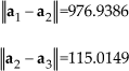
\begin{array}{l} ‖ a_{1} - a_{2} ‖ =976 . 9386 \\ ‖ a_{2} - a_{3} ‖ =115 . 0149 \end{array}

The side lengths of the mobile platform:

\begin{array}{l} ‖ b_{1} - b_{2} ‖ =651 . 2924 \\ ‖ b_{2} - b_{3} ‖ =76 . 6766 \end{array}

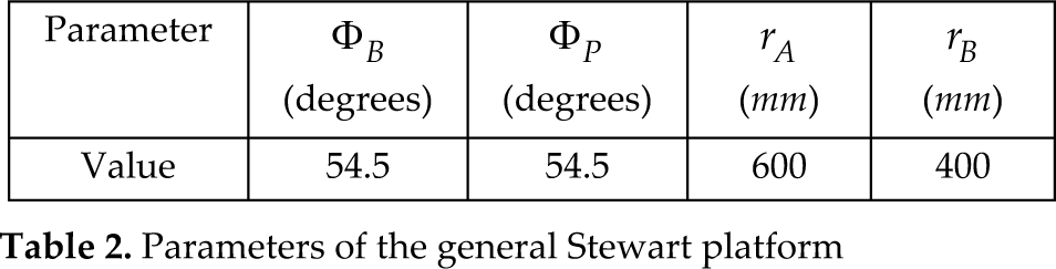
The radius of the base circumscribed in a circle and the distributing angles of the manipulator are written in Table 2.

Table 2.

Parameters of the general Stewart platform

Parameter	Φ_B (degrees)	Φ_P (degrees)	r_A (mm)	r_B (mm)
Value	54.5	54.5	600	400

Therefore, the coordinates of the joints on the base platform are:

\begin{array}{l} a_{1} (- 275.9340, 532.7855, 0), \\ a_{2} (- 534.0014, 273.5734, 0), \\ a_{3} (84.6809, - 593.9942, 0), \\ a_{4} (593.6136, - 434.4520, 0), \\ a_{5} (413.8253, - 434.4520, 0), \\ a_{6} (- 275.9340, 532.7855, 0) \end{array}

The workspace of the platform has been defined as a cube centred at Cartesian coordinates [x,y,z] = [0,0,976.3450], see Fig. 4. Orientation angle δ has been defined as a zero constant value (degrees). In this form the elements of x˜ can be written as

\begin{array}{l} x \in [+ 60, - 60] \\ y \in [+ 60, - 60] \\ z \in [+ 40, - 40] \\ α \in [+ 20, - 20] \\ β \in [+ 20, - 20] \end{array}

(13)

Figure 4.

A scheme showing the prescribed workspace for the Stewart platform

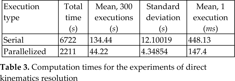
Using the hybrid algorithm described in Section 3, several experiments were run. The proposal was programmed in C and compiled with a GNU compiler. All experiments were executed in the SO Linux Open Suse version 12.1 in a CPU with 3.4 Ghz, 4 cores and 16Gb of RAM. For the hybrid optimizer, we considered two kinds of implementations, serial and parallelized executions. This code was parallelized with openMP, by executing the evaluation process using a Dogleg algorithm. In particular, serial experiments consisted of a set of 300 serial executions, repeated 10 times for statistical purposes. In the same form, the parallelized experiments consisted of a set of 300 parallelized executions which were repeated 10 times. The times of executions for experiments are shown in Table 3. From Table 3 it can be seen that by using four cores, the time for parallelized executions (evaluations with the Dogleg algorithm) is reduced 67.11% with respect to serial executions. Today, there are computers for high performance computing with 96 cores that could offer more reduction of computation times.

Table 3.

Computation times for the experiments of direct kinematics resolution

Execution type	Total time (s)	Mean, 300 executions (s)	Standard deviation (s)	Mean, 1 execution (ms)
Serial	6722	134.44	12.10019	448.13
Parallelized	2211	44.22	4.34854	147.4

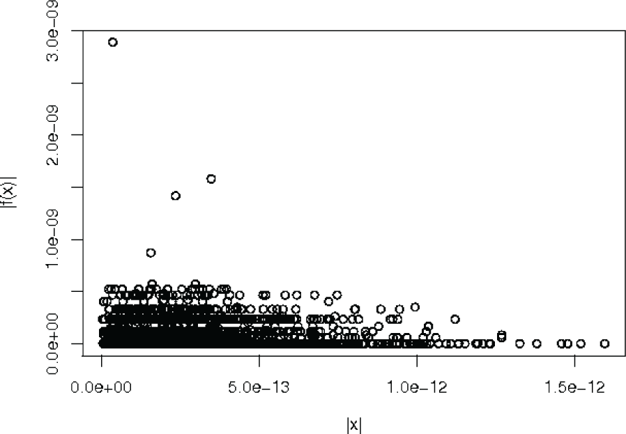
In order to show the proposal performance in terms of its precision, we compute the Euclidean norm of the differences between the desired pose variables (x) and the computed pose variables (x*). Figure 5 shows a mapping between the norm of pose's variables differences and the norm of the solver (desired precision of the hybrid optimizer) for the executions with serial implementation, where |x| represents the norm of pose variables differences and |f(x)| the norm of the optimizer. The norm of the solver was computed by using the Minpack enorm function [38]. The maximum precision that the solver can achieve is 2.22044604926e-16, i.e., the desired precision for all executions.

Figure 5.

A map of the norm of pose's variables differences and the norm of the hybrid optimizer for serial implementation

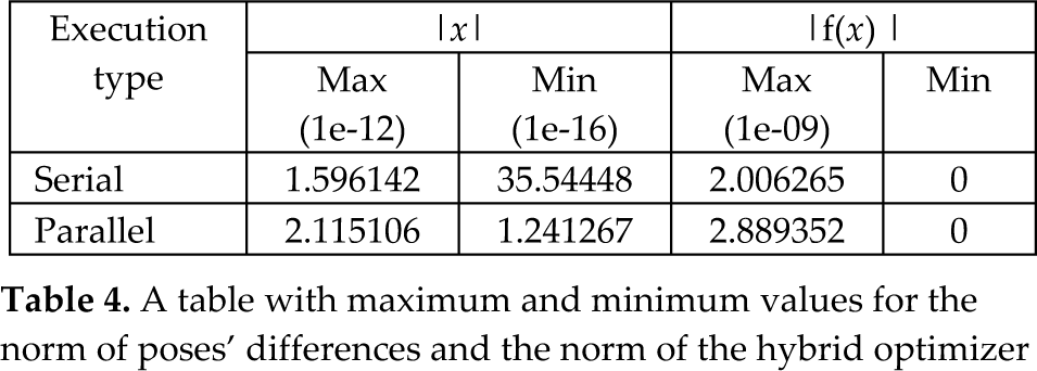
In the same way, Figure 6 shows this mapping for the experiments with a set of parallelized executions. From these figures it can be seen that the differences between the computed poses and the desired ones remain below 1.5e-12 for serial executions and below 2.5e-12 for the case of parallelized executions. In resume, Table 4 shows the maximum and minimum values for these differences, we can observe that in both cases the desired precision is achieved.

Figure 6.

A map of the norm of pose's variables differences and the norm of the hybrid optimizer for parallelized executions

Table 4.

A table with maximum and minimum values for the norm of poses' differences and the norm of the hybrid optimizer

Execution type	\|x\|		\|f(x)\|
Execution type	Max (1e-12)	Min (1e-16)	Max (1e-09)	Min
Serial	1.596142	35.54448	2.006265	0
Parallel	2.115106	1.241267	2.889352	0

From Figure 7, we can see that the two implementations have similar dispersions and data distribution. For both distributions, 75% of data for pose differences are below 6.66e-13, approximately. In the same form, we can identify some atypical values, but these always belong to the desired range of precision.

Figure 7.

A boxplot graph comparing hybrid optimizer precision, left for serial implementation and right for parallelized implementation

These results are confirmed by the histograms of Figures 8 and 9, for serial and parallelized experiments, respectively. From these histograms we can assume that a lot of executions for solving the direct kinematics of the general Stewart platform are achieved with a high precision (differences between the desired poses and the computed ones below 1.5e-12).

Figure 8.

A histogram of the norm of pose differences for serial executions

Figure 9.

A histogram of the norm of pose differences for parallelized executions

4.3 Confidence about the Global Minimum

In this section we present strong arguments about the confidence of the global optimum found by our algorithm. The first argument is about the verification of a solution once we have found it. The second argument is about exploration in order to find such a solution. The second order optimality conditions [35] state that if the gradient equals 0 in x*, ∇ F(x*) = 0, and the Hessian of the function is greater than 0, ∇²F(x*) >0. Then we can ensure that a local minimum of the function is found. These conditions are ensured by the Dogleg method used for local minimization. In addition, for this case, or in general, when solving systems of non-linear equations by intending to minimize the square norm of the error, the following argument holds: if the image of a proposed solutionis 0, that is to say F(x̂) = 0, then we certainly know that x is a solution of the system of equations because it satisfies such a system. For example, suppose a 2-variable, 2-equation system as follows: f₁(x₁,x₂) = c₁,f ₂(x₁,x₂) = c₂. The error vector is: [f₁(x₁,x₂)-c₁,f₂(x₁,x₂)-c₂]. The norm of the error is given as the function F as follows:

F (x_{1}, x_{2}) = \sqrt{{(f_{1} (x_{1}, x_{2}) - c_{1})}^{2} + {(f_{2} (x_{1}, x_{2}) - c_{2})}^{2}} .

If we found such a point (x̂₁,x̂₂), that (x̂₁,x̂₂), then (f₁(x̂₁,x̂₂)-c₁)=0, and (f₂(x̂₁,x̂₂)-c₁)=0, in consequence: f₁(x̂₁,x̂₂)=c₁,f₂(x̂₁,x̂₂)-c₂. This means that we can ensure that the global solution of the system has been found. In our experiment we have verified that F(x̂) = 0; for the direct kinematics system in practice it is not easy to solve the direct kinematics, but it is easy to verify if a point x̂ is a solution. In other words, it is not easy to find x̂, but once we have verified that F(x̂) = 0 we can ensure that it is a global optimum.

The argument just stated tackles the verification of a solution when it is found; the second argument is about the exploration, when looking for the actual global optimum. Consider that the optimum (the solution of the direct kinematics) is in a “convex” region or an attractor that represents 5% of the search space, that is to say, if we can pose a point in this region, then we have found the optimum. If we sample a single candidate solution using a uniform distribution on the search space, the probability of posing such a candidate solution in the attractor region is 0.05, consequently the probability of not sampling the region is 0.95. Even though this probability is large, notice that if we sample two candidate solutions, the probability of “not” sampling the region is 0.952, if we sample n candidate solutions, then the probability of not sampling the attractor region is 0.95^npop when using a uniform distribution (the first generation of the EDA). In our examples we use n_pop =100 and the number of points randomly drawn is from 100 to 15000, according to the generation when the solution is found. Then, for the hypothetical example of an attractor of 5% of the search space, the probability of not sampling such a region using a uniform distribution is from 0.95¹⁰⁰=0.00592 to 0.95¹⁵⁰⁰ ≈ 0. These probabilities are computed by considering a uniform distribution. In our experiments we have tested (statistically) that in most cases our algorithm performs better than a uniform distribution, therefore our probabilities of “not sampling” the optimum could be smaller than those of the uniform distribution. In the same vein, we have verified that the solution found for our algorithm is always a global minimum according the first argument of this section.

5. Conclusion

This article proposes a hybrid method to solve the direct kinematics of general Stewart platforms, which can directly generate a unique solution. The proposal combines a state of the art optimizer which is not based in derivatives which are widely used and also a state of the art optimizer for convex functions. The first one avoids becoming trapped in local minima, providing well performed starting points for the second one, which provides a high precision solution efficiently (in a convex region). The novelty of our proposal is the combination of both strategies and the use of them to solve a hard optimization real world problem. We present statistical evidence about the method in order to argue that it performs better than a “blind search”, that is to say our method performs better than using random starting points. Notice that this is quite important if we are looking for the automation of the direct kinematics solver, avoiding the need for user intervention and a priori knowledge. Additionally, our proposal is highly parallelizable, which can lead us to reduce computation time by exploiting the resources of today's high performance computers. This proposal can be used to solve non-convex global optimization problems.

Footnotes

6. Acknowledgments

The authors would like to thank PROMEP-Mexico for supporting part of this project through grant 103.5/10/5489.

References

Merlet

J. P.

, Parallel Robots. Springer, Dordrecht, The Netherlands, 2006.

Stewart

, “A Platform with Six Degrees of Freedom,” Proceedings of the Institution of Mechanical Engineers, vol. 180, num. 15, pp. 371–386, 1965.

Gough

V. E.

Whitehall

S. G.

, “Universal Tyre Test Machine,” in FISITA Ninth International Technical Congress, 1962, pp. 117–137.

Zhuang

Roth

, “Method for Kinematic Calibration of Stewart Platforms,” Journal of Robotic Systems, vol. 10, num. 3, pp. 391–405, 1993.

Masory

Wang

Zhuang

, “On the Accuracy of a Stewart Platform-part {II}: Kinematic Calibration and Compensation,” in IEEE Int. Conf. on Robotics and Automation, Atlanta, 1996, pp. 725–731.

Patel

A. J.

Ehmann

K. F.

, “Volumetric Error Analysis of a Stewart Platform based Machine Tool,” Annals of the CIRP, vol. 46, num. 1, pp. 287–290, 1997.

Shih-Ming

Ehman

K. F.

, “Error Model and Accuracy Analysis of a Six-DOF Stewart Platform,” Journal of Manufacturing Science and Engineering, vol. 124, pp. 286–295, 2002.

Hernandez-Martinez

Ceccarelli

Carbone

Lopez-Cajun

Jauregui-Correa

J. C.

, “A Characterization of Milli-CaTraSys System, a Parallel Manipulator for Measuring Purposes,” Mechanism Based Design of Structures and Machines an International Journal, vol. 38, pp. 25–49, 2010.

Merlet

J. P.

, “Singular Configurations of Parallel Manipulators and Grassman Geometry,” International Journal of Robotics Research, vol. 8, num. 5, pp. 45–56, 1989.

10.

Merlet

J. P.

, “Solving the Forward Kinematics of a Gough-type Parallel Manipulator with Interval Analysis,” International Journal of Robotics Research, vol. 23, num. 3, pp. 221–235, 2004.

11.

Nanua

Waldron

K. J.

Murthy

, “Direct Kinematic Solution of a Stewart Platform,” IEEE Transactions on Robotics and Automation, vol. 6, num. 4, pp. 438–444, 1990.

12.

Waldron

K. J.

Raghavan

Roth

, “Kinematics of a Hybrid Series-parallel Manipulator System,” Journal of Dynamic Systems Measuring and Control, vol. 111, num. 2, pp. 211–221, 1989.

13.

, Ed., An Approach for Direct Kinematics of a Parallel Manipulator Robot (ISIA 2010, CCIS 86). Berlin: Springer-Verlag Heidelberg, 2011, pp. 524–528.

14.

Innocenti

Parenti-Castelli

, Direct Kinematics of the 6-4 fully Parallel Manipulator with Position and Orientation Decoupled. Kluwer Academic, Amsterdam, 1992.

15.

Wampler

C. W.

, “Forward Displacement Analysis of General Six-in-parallel SPS (Stewart) Platform Manipulators using Soma Coordinates,” Mechanism and Machine Theory, vol. 31, num. 3, pp. 331–337, 1996.

16.

Xiong

, Eds., A Method for Forward Kinematics of Stewart Platform Manipulators(ICIRA 2008,part I, LNAI 5314). Berlin: Springer-Verlag Heidelberg, 2008, pp. 171–178.

17.

Innocenti

, “Forward Kinematics in Polynomial form of the General Stewart Platform,” ASME Journal of Mechanical Design, vol. 123, pp. 254–260, 2001.

18.

Lee

T. Y.

Shim

J. K

, “Forward Kinematics of the General 6-6 Stewart Platform using Algebraic Elimination,” Mechanism and Machine Theory, vol. 36, pp. 1073–1085, 2001.

19.

Gan

Liao

Dai

J. S.

Wei

, “Forward Displacement Analysis of the General 6-6 Stewart Mechanism using Grobner Bases,” Mechanism and Machine Theory, vol. 44, pp. 1640–1647, 2009.

20.

Huang

Liao

Wei

, “Closed-form Forward Kinematics for a Symmetrical 6-6 Stewart Platform using Algebraic Elimination,” Mechanism and Machine Theory, vol. 45, pp. 327–334, 2010.

21.

Zanganeh

K. E.

Angeles

, “Real-time Direct Kinematics of General Six-degree-of-freedom Parallel Manipulators with Minimum-sensor Data,” Journal of Robot Systems, vol. 12, num. 12, pp. 833–844, 1995.

22.

Dieudonne

J. E.

Parrish

R. V.

Bardusch

R. E.

, An Actuator Extension Transformation for a Motion Simulator and an Inverse Transformation Applying Newton-Raphson's, NASA Langley Research Center, Hampton, VA, Tech. Rep. NASA TND-7067, 1972.

23.

Merlet

J. P.

, “Direct Kinematics of Parallel Manipulator,” IEEE Transactions on Robot Automation, vol. 9, num. 6, pp. 842–846, 1993.

24.

Liu

Lewis

F. L.

Fitzgerald

, “Solution of Nonlinear Kinematics of a Parallel-link Constrained Stewart Platform Manipulator,” Circuits Systems Signal Process, vol. 3, pp. 167–183, 1994.

25.

Parikh

P. J.

Lam

S. Y.

, “A Hybrid Strategy to Solve the Forward Kinematics Problem in Parallel Manipulators,” IEEE Transactions on Robotics, vol. 21, num. 1, pp. 18–25, 2005.

26.

Geng

Haynes

L. S.

, “Neural Network Solution for the Forward Kinematics Problem of a Stewart Platform,” Robotics, Computing and Integrated Manufacturing, vol. 9, num. 6, pp. 485–495, 1992.

27.

Yee

C. S.

Lim

K. B.

, “Forward Kinematics Solution of Stewart Platform using Neural Networks,” Neurocomputing, vol. 16, num. 4, pp. 333–349, 1997.

28.

Parikh

P. J.

Lam

, “Solving the Forward Kinematics Problem in Parallel Manipulators using an Iterative Artificial Neural Network Strategy,” International Journal of Advanced Manufacturing and Technology, vol. 40, pp. 595–606, 2009.

29.

Ghasemi

Eghtesad

Farid

, “Neural Network Solution for Forward Kinematics Problem of Cable Robots,” Journal of Intelligent and Robotic Systems, vol. 60, pp. 201–215, 2010.

30.

Zhuang

Huang

, “Optimal Planning of Robot Calibration Experiments by Genetic Algorithms,” in IEEE International Conference on Robotics and Automation, Minneapolis, 1996, pp. 22–28.

31.

Omran

El-Bayiumi

Kassem

, “Genetic Algorithm Based Optimal Control for a 6-DOF Non Redundant Stewart Manipulator,” International Journal of Mechanical Systems Science and Engineering, vol. 2, num 2, pp. 73–75, 2008.

32.

Rolland

Chandra

, “On Solving the Forward Kinematics of the 6-6 General Parallel Manipulator with an Efficient Evolutionary Algorithm,” in 18th CISM-IFToMM Symposium on Robot Design, Dynamics, and Control, Udine, pp. 117–124, 2010.

33.

Cabrera

J. A.

Castillo

J. J.

Nadal

Ortiz

Simon

, “Synthesis of Mechanisms with Evolutionary Techniques,” in Proceedings of Eucomes 08, The Second European Conference on Mechanism Science, Cassino, 2008, pp. 21–25.

34.

Gosselin

, Kinematic Analysis, Optimization and Programming of Parallel Robotic Manipulators. Ph.D. Thesis, McGill University, 1988.

35.

Nocedal

Wright

, Numerical Optimization. Springer, Second Edition, 2006.

36.

Larrañaga

Lozano

J. A.

, Estimation of Distribution Algorithms: A New Tool for Evolutionary Computation. Kluwer Academic Publishers, Norwell, MA, USA, 2001.

37.

Efron

Tibshirani

R. J.

, An Introduction to the Bootstrap. Chapman and Hall, Monographs on Statistics and Applied Probability, New York, 1993.

38.

Moré

J. J.

Sorensen

D. C.

Hillstrom

K. E.

, and Garbow

B. S.

, The MINPACK Project, in Sources and Development of Mathematical Software, Cowell

W. J.

, ed., Prentice-Hall,pp. 88–111, 1984.

Towards a Robust Solution of the Non-Linear Kinematics for the General Stewart Platform with Estimation of Distribution Algorithms

Abstract

Keywords

1. Introduction

2. Problem Formulation: Non-linear Kinematics of the Stewart Platform

3. Implementation of the Hybrid Optimizer

4. Experiments and Results

4.1 Contrasting EDA-based Gaussian and Uniform Distributions

4.2 A Numerical Example

4.3 Confidence about the Global Minimum

5. Conclusion

Footnotes

6. Acknowledgments

References