Sage Journals: Discover world-class research

Abstract

An adaptive control approach is proposed for trajectory tracking and obstacle avoidance for mobile robots with consideration given to unknown sliding. A kinematic model of mobile robots is established in this paper, in which both longitudinal and lateral sliding are considered and processed as three time-varying parameters. A sliding model observer is introduced to estimate the sliding parameters online. A stable tracking control law for this nonholonomic system is proposed to compensate the unknown sliding effect. From Lyapunov-stability analysis, it is proved, regardless of unknown sliding, that tracking errors of the controlled closed-loop system are asymptotically stable, the tracking errors converge to zero outside the obstacle detection region and obstacle avoidance is guaranteed inside the obstacle detection region. The efficiency and robustness of the proposed control system are verified by simulation results.

Keywords

Wheeled mobile robot Obstacle avoidance Potential function Adaptive control Unknown sliding parameters Sliding model observer

1. Introduction

The past last few decades have witnessed an ambitious research effort in the area of motion control of mobile robot (see [1 –14] and the references therein). These works always assume that the mobile robots are subject to ‘pure rolling without slipping’, namely they keep nonholonomic constraints for controlling mobile robots. However, sliding effects have a critical influence on the performance of mobile robots that cannot be neglected. It means that we should deal with the mobile robot model with sliding induced from perturbed non-homonymic constraints for more a practical consideration. With this in mind, some researchers have studied approaches for controlling mobile robots considering skidding and slipping [15 –19]. In [15, 16], only the skidding effect was considered. Wang and Low [17] proposed models of wheeled mobile robots (WMRs) considering the sliding of both wheels and analysed their controllability according to the manoeuvrability of mobile robots. They also designed controllers for path following and the tracking of mobile robots that took sliding into consideration [18,19]. However, the information on skidding and slipping should be measured by a global positioning system (GPS), but only kinematics was used to design the controllers in [18,19]. Besides, the works [17 –19] did not include any ideas for obstacle avoidance for mobile robots in the presence of wheel sliding.

Owing to the difficulty in handling both tracking and obstacle avoidance using one controller, there are few results available on the tracking control problem for nonholonomic mobile robots with obstacle avoidance, even though the problem is practical and important. Recently, some research work has investigated the problem on the kinematic level [20,21] and on the dynamic level [22 –24]. The control approaches reported in [20,22] are commonly designed into tracking controllers with obstacle avoidance capability by using position tracking errors without coordinate transformation. However, some methods were developed without considering skidding and slipping effects [20 –22] and obstacle avoidance is not considered in [23]. In [24], an adaptive controller is designed for trajectory tracking and obstacle avoidance in mobile robots and considers unknown sliding on the dynamic level by a backstepping approach. However, the design process of this controller is very complex and its implementation is not easy. This point motivates us to extend the study on tracking and obstacle avoidance in the presence of unknown sliding.

The main contributions of our work are the design of an adaptive control system, on the kinematics level, for tracking and obstacle avoidance for a class of mobile robots in the presence of unknown sliding. More specifically, in the theoretical part of this paper, we design a controller that guarantees tracking with bounded error and obstacle collision avoidance for mobile robot systems with unknown sliding. We assume that each robot knows its position and can detect the presence of any object within a given range. We apply this result to the control of the mobile robot system. Firstly, a kinematic model of mobile robots considering the influence of sliding is established where sliding is modelled as three time-varying parameters. Secondly, the time-varying sliding parameters are estimated by the sliding model observer online. The proposed adaptive controller is designed using Lyapunov design techniques where the angular velocities of the wheels are considered as the immediate controls to deal with unmatched sliding at the robot kinematics level. By using the Lyapunov stability approach with a potential function, we prove that the tracking errors of a controlled closed-loop system can converge asymptotically. The tracking errors converge to zero outside the obstacle detection region and no-collision between the robot and the obstacle is guaranteed inside the obstacle detection region, regardless of unknown sliding. Finally, simulation results are included to demonstrate the effectiveness of the proposed control approach.

This paper is organised as follows. In Section 2, we present the kinematic model of mobile robots considering the sliding influence, where sliding is modelled as three time-varying parameters. In Section 3, the sliding observer is employed to estimate sliding parameters and is introduced in detail. In Section 4, a controller is designed that guarantees tracking and obstacle avoidance for the mobile robot in the presence of sliding and the stability of the proposed control system is analysed. Simulation results are discussed in Section 5. Finally, Section 6 gives some conclusions.

2. Kinematic model of a wheeled mobile robot in the presence of sliding

A simple differentially steered WMR is shown as Fig.1. It has two differential driving wheels and two back caster wheels. The two driving wheels are powered independently by two DC servo motors respectively and have the same wheel radius.

Figure 1.

Tracked mobile robot with two independent driving wheels

To describe the motion features of a tracked mobile robot simply and rigorously in the general plane of motion, a fixed reference coordinate frame F₁(X,Y) and a moving coordinate frame F₂ (x, y) which attaches to the robot body with the origin at the geometric centre O, are defined

The linear velocities of left and right driving wheels of mobile robot without sliding are represented as follows

\begin{matrix} v_{L} = r ω_{L} \\ v_{R} = r ω_{R} \end{matrix}

(1)

where ω_L and ω_R are the angular velocities of the left and right wheels respectively, r is radius of the wheels. The longitudinal slip ratios of the left and right wheels of a tracked mobile robot are defined as follows [25]

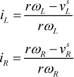
\begin{matrix} i_{L} = \frac{r ω_{L} - v_{L}^{s}}{r ω_{L}} \\ i_{R} = \frac{r ω_{R} - v_{R}^{s}}{r ω_{R}} \end{matrix}

(2)

where v_L^s and vs are respectively, the linear velocities of the left and right wheels of the mobile robot in the presence of wheel slipping. The range of the longitudinal slip ratio i_R and i_L lies between [0,1]. The lateral sliding ratio of a tracked mobile robot is defined as [25]:

δ = \tan α

(3)

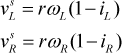
where α is the lateral sliding angle of a mobile robot (see Fig.1). From Equation (2), the linear velocities of the left and right wheels of the mobile robot in the presence of wheel slipping are given as:

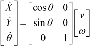
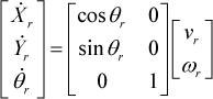
\begin{array}{l} v_{L}^{s} = r ω_{L} (1 - i_{L}) \\ v_{R}^{s} = r ω_{R} (1 - i_{R}) \end{array}

(4)

In the coordinate frame F₁ (X, Y) and in the absence of wheel slipping the kinematic model of the WMR is described by:

[\begin{matrix} \dot{X} \\ \dot{Y} \\ \dot{θ} \end{matrix}] = [\begin{matrix} \cos θ & 0 \\ \sin θ & 0 \\ 0 & 1 \end{matrix}] [\begin{matrix} v \\ ω \end{matrix}]

(5)

In the coordinate frame F₂(x,y) a suitable model with sliding can be written as:

\begin{array}{l} \dot{x} = \frac{r ω_{L} (1 - i_{L}) + r ω_{R} (1 - i_{R})}{2} \\ \dot{y} = - \frac{r ω_{L} (1 - i_{L}) + r ω_{R} (1 - i_{R})}{2} δ \\ \dot{θ} = \frac{r ω_{R} (1 - i_{R}) - r ω_{L} (1 - i_{L})}{b} \end{array}

(6)

where b is the distance between the two driving wheels. As shown in Fig.1, the relationship of the coordinate transformation from F₁(X,Y) to F₂ (x, y) is given by

[\begin{matrix} X \\ Y \end{matrix}] = [\begin{matrix} \cos θ & - \sin θ \\ \sin θ & \cos θ \end{matrix}] [\begin{matrix} x \\ y \end{matrix}]

(7)

From equations (6) and (7), in the coordinate frame F₁(X,Y), the kinematic model of the differential WMR with sliding is described as follows:

\begin{array}{l} \dot{X} = \frac{r ω_{L} (1 - i_{L}) + r ω_{R} (1 - i_{R})}{2} (\cos θ + δ \sin θ) \\ \dot{Y} = \frac{r ω_{L} (1 - i_{L}) + r ω_{R} (1 - i_{R})}{2} (\sin θ - δ \cos θ) \\ \dot{θ} = \frac{r ω_{R} (1 - i_{R}) - r ω_{L} (1 - i_{L})}{b} \end{array}

(8)

where [X, Y, θ] ^T is the posture vector of mobile robot, θ is the heading angle of the WMR (the angle that is between the motion direction of robot and the positive direction of the X axis).

If $\dot{x} = \frac{r ω_{L} (1 - i_{L}) + r ω_{R} (1 - i_{R})}{2}$ is defined as the longitudinal speed of the WMR in Fig.1, then, Equation (8) can be rewritten as

\begin{array}{l} \dot{X} = \dot{x} (\cos θ + δ \sin θ) \\ \dot{Y} = \dot{x} (\sin θ - δ \cos θ) \\ \dot{θ} = \frac{2 \dot{x}}{b} - \frac{2 r}{b} ω_{L} (1 - i_{L}) = \frac{- 2 \dot{x}}{b} + \frac{2 r}{b} ω_{R} (1 - i_{R}) \end{array}

(9)

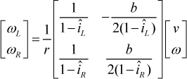
If we define an auxiliary control input ū= [v, ω]^T, then the relationship between the auxiliary control input and effective control input u = [ω_L,ω_R]^T is regarded as:

\begin{array}{l} \bar{u} = [\begin{matrix} v \\ ω \end{matrix}] = [\begin{matrix} \frac{r (1 - i_{L}) ω_{L} + r (1 - i_{R}) ω_{R}}{2} \\ \frac{- r (1 - i_{L}) ω_{L} + r (1 - i_{R}) ω_{R}}{b} \end{matrix}] \\ = T [\begin{matrix} ω_{L} \\ ω_{R} \end{matrix}] = T u \end{array}

(10)

where the matrix $T = r [\begin{matrix} \frac{1 - i_{L}}{2} & \frac{1 - i_{R}}{2} \\ \frac{- (1 - i_{L})}{b} & \frac{1 - i_{R}}{b} \end{matrix}]$ , is a nonsingular matrix. From Equation (10), effective control input u = [ω_L, ω_R]^T can be obtained as follows:

[\begin{matrix} ω_{L} \\ ω_{R} \end{matrix}] = T^{- 1} [\begin{matrix} v \\ ω \end{matrix}] = \frac{1}{r} [\begin{matrix} \frac{1}{1 - i_{L}} & - \frac{b}{2 (1 - i_{L})} \\ \frac{1}{1 - i_{R}} & \frac{b}{2 (1 - i_{R})} \end{matrix}] [\begin{matrix} v \\ ω \end{matrix}]

(11)

Equation (8) can be written as:

[\begin{matrix} \dot{X} \\ \dot{Y} \\ \dot{θ} \end{matrix}] = [\begin{matrix} \cos θ + δ \sin θ & 0 \\ \sin θ - δ \cos θ & 0 \\ 0 & 1 \end{matrix}] [\begin{matrix} v \\ ω \end{matrix}]

(12)

As can be seen from Equation (8), to solve the tracking control problem of a WMR with unknown sliding parameters i_R,i_L and δ, the top priority is to estimate the time-varying sliding parameters online and then to design the tracking controller on the basis of the sliding parameter estimations.

3. Robot sliding parameter estimation schemes

3.1 Design of nonlinear sliding model observer

The SMO (Sliding Model Observer) is a popular approach for state estimation, since it can deal with uncertainty in the system [26]. In this paper, an SMO [26 –29] is designed to estimate sliding parameters, based on the kinematics model of the robot, sensor feedback of the robot's trajectory and the driving wheel speeds. Due to the inherent non-linear nature of the robot kinematics equations, it is a complex problem to obtain an estimation of the robot sliding parameters. The kinematics equations have to be linearized at a nominal trajectory when a linear estimator such as the Kalman Filter is applied to estimate the slipping parameters. Furthermore, measurements from inertia sensors include significant noise, it is very important for the observer to be robust against noise and model uncertainty. With an SMO, the control action switches from one value to another in finite time and this may cause chattering problems; to avoid this effect, the discontinuous terms go through a Low Pass Filter. An SMO is used to estimate the motor torque based on a single-input, single-output dynamics system as in [26]. In [28] two variables: disturbance and steering angle are estimated using an SMO, however the chattering is unavoidable due to the switching of sign function. The paper applies this approach to the multi-input, multi-output dynamics system and reduces the chattering by passing discontinuous terms from the observers through a low pass filter.

The observer takes the form as follows:

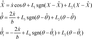
\begin{array}{l} \dot{\hat{X}} = \dot{x} \cos θ + L_{1} sgn (X - \hat{X}) + L_{2} (X - \hat{X}) \\ \dot{\hat{θ}} = \frac{2 \dot{x}}{b} + L_{3} sgn (θ - \hat{θ}) + L_{2} (θ - \hat{θ}) \\ {\dot{\hat{θ}}}_{1} = - \frac{2 \dot{x}}{b} + L_{4} sgn (θ - {\hat{θ}}_{1}) + L_{2} (θ - {\hat{θ}}_{1}) \end{array}

(13)

where L_i > 0,1 = 1,2, … 4 are sliding model gains, $\overset{^̇}{X}$ is the estimated velocity X of the robot, $\dot{\hat{θ}}$ is the estimated directional speed of the robot and yaw rate, $\dot{\hat{θ}}$ is the estimated directional speed of the robot, sign function:

$sgn (x) = {\begin{matrix} \begin{matrix} - 1 & x \leq 0 \end{matrix} \\ \begin{matrix} 1 & x > 0 \end{matrix} \end{matrix}, {\dot{\hat{θ}}}_{1}$ , is used for designing an appropriate sliding surface which stabilizes all the posture variables.

Errors are defined as $\tilde{X} = X - \hat{X}$ , $\tilde{θ} = θ - \hat{θ}$ and $\tilde{θ} = θ - \hat{θ}$ and ${\tilde{θ}}_{1} = θ_{1} - {\hat{θ}}_{1}$ . By subtracting Equation (9) from (13) the following error dynamics can be obtained as:

\begin{array}{l} \dot{\tilde{X}} = δ \dot{x} \sin θ - L_{1} sgn (X - \hat{X}) - L_{2} (X - \hat{X}) \\ \dot{\tilde{θ}} = - \frac{2 r}{b} ω_{L} (1 - i_{L}) - L_{3} sgn (θ - \hat{θ}) - L_{2} (θ - \hat{θ}) \\ {\dot{\tilde{θ}}}_{1} = \frac{2 r}{b} ω_{R} (1 - i_{R}) - L_{4} sgn (θ - {\hat{θ}}_{1}) - L_{2} (θ - {\hat{θ}}_{1}) \end{array}

(14)

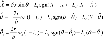
The error dynamics should converge to the sliding surface in a finite time by the appropriate choice of sliding gains, $X \to \hat{X}$ , $θ \to \hat{θ}$ , $θ \to \hat{θ}$ , then the equations (14) are reduced to:

\begin{array}{l} δ \dot{x} \sin θ - L_{1} sgn (X - \hat{X}) - L_{2} (X - \hat{X}) \approx 0 \\ - \frac{2 r}{b} ω_{L} (1 - i_{L}) - L_{3} sgn (θ - \hat{θ}) - L_{2} (θ - \hat{θ}) \approx 0 \\ \frac{2 r}{b} ω_{R} (1 - i_{R}) - L_{4} sgn (θ - {\hat{θ}}_{1}) - L_{2} (θ - {\hat{θ}}_{1}) \approx 0 \end{array}

(15)

If the driving wheels angular velocities ω_L, ω_R are measurable, the robot trajectory and sliding gains L₁, L₂, L₃, L₄ are given. Moreover, a low pass filter is applied to reduce the chattering of the SMO, then the sliding parameter estimations $\hat{δ}, {\hat{i}}_{L}, {\hat{i}}_{R}$ can be calculated as follows:

\begin{array}{l} \hat{δ} = \frac{L_{1} {(sgn (X - \hat{X}))}_{L P F}}{\dot{x} \sin θ} \\ {\hat{i}}_{L} = 1 + \frac{b}{2 r ω_{L}} L_{3} (sgn (θ - \hat{θ}))_{L P F} \\ {\hat{i}}_{R} = 1 - \frac{b}{2 r ω_{R}} L_{4} (sgn (θ_{1} - {\hat{θ}}_{1}))_{L P F} \end{array}

(16)

where (·) _LPF denotes an LPF (Low Pass Filter). The values of terms $L_{1} {(sgn (X - \hat{X}))}_{L P F}$ , $L_{3} {(sgn (θ - \hat{θ}))}_{L P F}$ , $L_{4} {(sgn (θ_{1} - {\hat{θ}}_{1}))}_{L P F}$ can be determined. A first-order low-pass filter is described in Fig.2

Figure 2.

Filtering processing of the estimation signal

The relationship between input u and output y of the LPF is given as:

γ \dot{y} + y = u, y (0) = u (0)

(17)

where $u = {[{\hat{i}}_{L}, {\hat{i}}_{R}, \hat{δ}]}^{T}$ and y = diag(γ₁,γ₂,γ₃), γ₁,γ₂,γ₃ > 0 the filter parameters, $L_{1} {(sgn (X - \hat{X}))}_{L P F}, L_{3} {(sgn (θ - \hat{θ}))}_{L P F}$ and $L_{4} {(sgn (θ_{1} - {\hat{θ}}_{1}))}_{L P F}$ are the state vectors of the low-pass filter, y is the output and γ is the filter time constant and a very small value that lies within 0 ≤ γ_i ≤ 1, i = 1,2,3.

3.2 Determination of switching gains

The switching gains L_i, i = 1,3,4 must be negative and large enough to satisfy the reaching condition of the sliding model. However, if it is too large, the chattering noise may lead to estimation errors. In this section, a proper selection of L_i, i = 1,3,4 is discussed.

In the following, the stability of the Sliding Model Observer (SMO) is discussed. The switching functions are defined as

s_{1} = X - \hat{X}, s_{2} = θ - \hat{θ}, s_{3} = θ_{1} - {\hat{θ}}_{1}

(18)

To ensure stability, the SMO dynamics must exhibit the following characteristics: (1) The error state must reach the sliding surface from an arbitrary point in error space in a finite time and (2) the error dynamics must be stable in some neighbourhood of the sliding surface. To enforce stability, the sliding mode gains should be chosen such that s_n · ṡ_n < 0, n = 1,2,3. It is shown in reference [26] that the error dynamics will converge in finite time if the conditions s_n · s_n <0, n = 1,2,3 are satisfied. Applying this approach:

\begin{array}{l} s_{1} {\dot{s}}_{1} = \dot{x} δ s_{1} \sin θ - L_{1} s_{1} sgn (s_{1}) - L_{2} s_{1}^{2} \\ \leq \dot{x} δ s_{1} \sin θ - L_{1} | s_{1} | \end{array}

(19)

From inequality (19), we know that if:

L_{1} > | \dot{x} δ \sin θ |

(20)

then s₁ · ṡ0. Similarly:

\begin{array}{l} s_{2} {\dot{s}}_{2} = \frac{2 r}{b} ω_{L} (1 - i_{L}) s_{2} - L_{3} s_{2} sgn (s_{2}) - L_{2} s_{2}^{2} \\ \leq \frac{2 r}{b} ω_{L} (1 - i_{L}) s_{2} - L_{3} | s_{2} | \end{array}

(21)

From inequality (21), we know that if:

L_{3} > \frac{2 r}{b} | ω_{L} (1 - i_{L}) |

(22)

then s₂ṡ₂ < 0. Thus sliding mode can be enforced if:

L_{4} > \frac{2 r}{b} | ω_{R} (1 - i_{R}) |

(23)

then s₃ṡ₃ < 0.

In practice, L₁ = |ẋ sin θ|, L₂ is a small positive number, L₃=4r/bω_L and L₄ =4r/bω_R. If the lateral sliding angle α is expected to be large (as is the case for steep side slopes with loose soil) the trial-and-error method can be used to determine L₁.

4. Design of the tracking and obstacle avoidance controller

4.1 Potential function for obstacle avoidance

To deal with the obstacle avoidance of mobile robots in the presence of sliding, we consider the following potential function: [24]

V_{o b} = {(\min {0, \frac{d_{r o}^{2} - L^{2}}{d_{r o}^{2} - l^{2}}})}^{2}

(24)

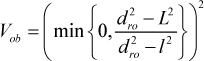
where l > 0 and L > 0 with L > l > b > 0 are radii of the avoidance and detection regions (see Fig.3), respectively. The parameter l can be chosen by considering the radius of the mobile robot body. The distance function d_ro between the robot and the obstacle is:

d_{r o} = \sqrt{{(X - X_{o})}^{2} + {(Y - Y_{o})}^{2}}

(25)

Figure 3.

Wheeled mobile robot with avoidance and detection region

with the obstacle position (X_o, Y_o). The function (24) goes to infinity as the boundary of the avoidance region for the mobile robot approaches the obstacle and is zero outside the detection region.

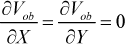
The partial derivatives of the potential function V_ob with respect to the X and Y coordinates which would be required in the controller design procedure can be defined as:

\frac{\partial V_{o b}}{\partial X} = {\begin{cases} \frac{4 (L^{2} - l^{2}) (d_{r o}^{2} - L^{2})}{{(d_{r o}^{2} - l^{2})}^{3}} (X - X_{o}), if l < d < L \\ 0, otherwise \end{cases}

(26)

\frac{\partial V_{o b}}{\partial Y} = {\begin{cases} \frac{4 (L^{2} - l^{2}) (d_{r o}^{2} - L^{2})}{{(d_{r o}^{2} - l^{2})}^{3}} (Y - Y_{o}), if l < d < L \\ 0, otherwise \end{cases}

(27)

Assumption 1: The reference trajectory is smooth and satisfies:

| e_{3} | \neq \frac{π}{2}, α - e_{3} \neq \frac{π}{2}

(28)

where e₃ =θ–θ_r is the orientation error and a is the lateral sliding angle of a mobile robot (in Fig.1). We define robot tracking errors: e₁ = X – X_r, e₂ = Y – Y_r.

Remark 1: Assumption 1 on the reference trajectory implies the following two conditions:

(1) Outside the detection region (d_ro > L) and for (e₁, e₂) ≠ (0,0) we have θ_r = A tan 2(–e₂, –e₁). The reference trajectory is such that it does not initiate sharp turns of 90° with respect to the current orientation of the robot. Note that this condition is not too restrictive since the robot can reorient itself on the spot if the condition is not satisfied and smoothness of the reference trajectory is a reasonable assumption in the case of robots subject to nonholonomic constraints.

(2) Inside the detection region (l<d_ro<L), we have $θ_{r} = A t a n 2 (- e_{2} - \frac{\partial V_{o b}}{\partial Y}, - e_{1} - \frac{\partial V_{o b}}{\partial X})$ .

The combination of obstacle position and reference trajectory might drive the robot into a singular configuration where Assumption 1 does not hold. One solution is to consider a perturbed desired orientation $θ_{r}$ , instead of the desired orientation θ_r whenever (Assumption 1) is not satisfied. In particular, a robot can modify the desired orientation when Assumption 1 is not satisfied; θ_r is replaced with the following perturbed version: ${\bar{θ}}_{r} = θ_{r} + \bar{ε}$ where $\bar{ε} \neq 0$ is some small perturbation value. This condition guarantees that the system avoids singularities and deadlocks.

4.2 Design of controller

4.2.1 Control objective

The control objective is to design an adaptive control law for mobile robots considering the kinematics (8) with unknown sliding so that:

1. Outside the detection region (d_ro ≥ L), the mobile robot tracks the reference trajectory generated by the following reference robot:

[\begin{matrix} {\dot{X}}_{r} \\ {\dot{Y}}_{r} \\ {\dot{θ}}_{r} \end{matrix}] = [\begin{matrix} \cos θ_{r} & 0 \\ \sin θ_{r} & 0 \\ 0 & 1 \end{matrix}] [\begin{matrix} v_{r} \\ ω_{r} \end{matrix}]

(29)

where X_r, Y_r and θ_r are the position and orientation of the reference robot and, v_r and ω_r are the linear and angular velocities of the reference robot.

2. Inside the detection region (l < d_ro < L), the mobile robot safely avoids obstacles under the influence of the reference trajectory Ẋ_r =Ẏ_r =0 and θ_r = A tan 2(–E_Y, –E_X) with:

{\begin{cases} E_{X} = X - X_{r} + \frac{\partial V_{o b}}{\partial X} \\ E_{Y} = Y - Y_{r} + \frac{\partial V_{o b}}{\partial Y} \end{cases}

(30)

while all other signals remain semi-globally uniformly ultimately bounded.

Remark 2: In the control objective, the reference trajectory remains constant inside the detection region, that is, Ẋ_r = Ẏ_r = 0 for l < d_ro < L. This means that when the mobile robot detects an obstacle in its trajectory, it keeps its reference to the last data received for a moment while trying to resolve the collision [24]. The reason for this choice is that collision avoidance has a higher priority than tracking, as a collision between the robot and obstacle could lead to system damage, which is more critical than temporary degeneration of tracking performance. Also, we define the desired orientation as θ_r=A tan2(–E_Y, –E_X) inside the detection region. The reason is that when the mobile robot detects the obstacle, the direction of motion is related to the reference trajectory, the robot position and the change of potential function.

Assumption 2: The reference velocity z_r =[v_r,ω_r]^T is bounded, where v_r > 0 is outside the detection region (d_ro ≥ L) and v_r =0 is inside the detection region (l < d_ro < L).

Remark 3: Assumption 2 is reasonable because this paper focuses on the trajectory tracking problem (i.e. v_r > 0) outside the detection region and the obstacle avoidance problem (i.e. v_r = 0 due to Ẋ_r=Ẏ_r=0) inside the detection region.

Assumption 3: From θ_r = A tan 2(–E_X, –E_Y), we can obtain:

{\dot{θ}}_{r} = \frac{E_{X} {\dot{E}}_{Y} - {\dot{E}}_{X} E_{Y}}{E_{X}^{2} + E_{Y}^{2}}

(31)

Hence:

{\hat{\dot{θ}}}_{r} = \frac{E_{X} {\hat{\dot{E}}}_{Y} - {\hat{\dot{E}}}_{X} E_{Y}}{E_{X}^{2} + E_{Y}^{2}}

(32)

where ${\hat{\dot{θ}}}_{r}$ is a sufficiently smooth estimation of ${\dot{θ}}_{r}$ . In practice E_X and E_Y are noisy signals and in order to perform this task and avoid the effects of the noisy measurements we make use of a numerical differentiation based on algebraic nonlinear estimation to obtain ${\hat{\dot{E}}}_{X}, {\hat{\dot{E}}}_{Y}$ . ${\hat{\dot{E}}}_{X}, {\hat{\dot{E}}}_{Y}$ are given as follows: [30]

{\begin{cases} {\hat{\dot{E}}}_{X} = - \frac{3!}{T^{3}} \int_{t - T}^{t} [2 T (t - τ) - T] E_{X} (τ) d τ \\ {\hat{\dot{E}}}_{Y} = - \frac{3!}{T^{3}} \int_{t - T}^{t} [2 T (t - τ) - T] E_{Y} (τ) d τ \end{cases}

(33)

where [t–T,t] is quite a short sliding time window. We assume that $| {\hat{\dot{θ}}}_{r} - {\dot{θ}}_{r} | \leq ε$ for some small positive ε. Note that most of the variables in ${\dot{θ}}_{r}$ can be measured, in fact we have:

| {\hat{\dot{θ}}}_{r} - {\dot{θ}}_{r} | = \frac{E_{X} ({\dot{E}}_{Y} - {\hat{\dot{E}}}_{Y}) - E_{Y} ({\dot{E}}_{X} - {\hat{\dot{E}}}_{X})}{E_{X}^{2} + E_{Y}^{2}}

(34)

where E_X, E_Y, $\sqrt{E_{X}^{2} + E_{Y}^{2}}$ can be computed using the state measurements and desired values. Then E_X, E_Y are smooth almost everywhere, we have $({\dot{E}}_{X} - {\hat{\dot{E}}}_{X}) ≃ ({\dot{E}}_{Y} - {\hat{\dot{E}}}_{Y}) ≃ o (T)$ and we can choose ε = o(T).

4.2.2 Design of controller

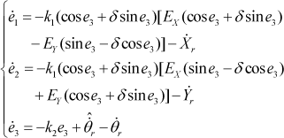
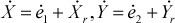
Define the tracking errors of a mobile robot as e₁ = X – X_r, e₂ =Y – Y_r, e₃ = θ–θ_r; the tracking error vectors of mobile robot are defined as e = [e₁, e₂,e₃]^T. From Equation (12), the error dynamic equation of a mobile robot is obtained as:

[\begin{matrix} {\dot{e}}_{1} \\ {\dot{e}}_{2} \\ {\dot{e}}_{3} \end{matrix}] = [\begin{matrix} v [\cos (e_{3} + θ_{r}) + δ \sin (e_{3} + θ_{r})] - {\dot{X}}_{r} \\ v [\sin (e_{3} + θ_{r}) - δ \cos (e_{3} + θ_{r})] - {\dot{Y}}_{r} \\ ω - {\dot{θ}}_{r} \end{matrix}]

(35)

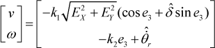
In the presence of sliding, we employ the Lyapunov direct method; the auxiliary control input is obtained as follows:

[\begin{matrix} v \\ ω \end{matrix}] = [\begin{matrix} - k_{1} \sqrt{E_{X}^{2} + E_{Y}^{2}} (\cos e_{3} + δ \sin e_{3}) \\ - k_{2} e_{3} + {\hat{\dot{θ}}}_{r} \end{matrix}]

(36)

where k₁ and k₂ are positive constants.

Now, if the sliding parameters i_R, i_L and δ that appear in (8) are unknown, we cannot choose directly the auxiliary control input as given by (36). Hence, we design a sliding model observer (13) to attain the control objective using estimations of i_R, i_L and δ. If î_L, î_R and $\hat{δ}$ denote the estimations of i_R, i_L and δ respectively, then, from Equation (36) we can obtain the auxiliary control input as:

[\begin{matrix} v \\ ω \end{matrix}] = [\begin{matrix} - k_{1} \sqrt{E_{X}^{2} + E_{Y}^{2}} (\cos e_{3} + \hat{δ} \sin e_{3}) \\ - k_{2} e_{3} + {\hat{\dot{θ}}}_{r} \end{matrix}]

(37)

where ${\hat{\dot{θ}}}_{r}$ is determined by equation(32), from Equation (11). Actual control input can also be obtained as follows:

[\begin{matrix} ω_{L} \\ ω_{R} \end{matrix}] = \frac{1}{r} [\begin{matrix} \frac{1}{1 - {\hat{i}}_{L}} & - \frac{b}{2 (1 - {\hat{i}}_{L})} \\ \frac{1}{1 - {\hat{i}}_{R}} & \frac{b}{2 (1 - {\hat{i}}_{R})} \end{matrix}] [\begin{matrix} v \\ ω \end{matrix}]

(38)

As can be seen from the above analysis, trajectory tracking and obstacle avoidance using a closed-loop control principle for the mobile robot can be described by the following scheme (See Fig.4).

Figure 4.

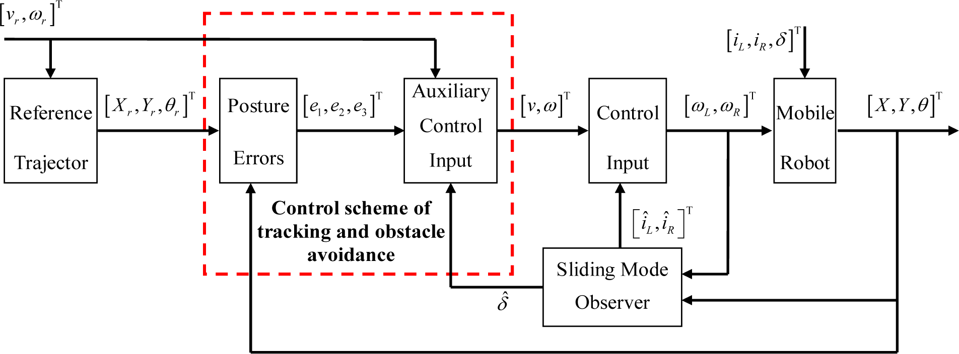
Mobile robot trajectory tracking and obstacle avoidance control principle scheme

4.2.3 Stability analysis of control system

Theorem 1: Consider system (12) and the reference trajectory described by (X_r, Y_r) that satisfies Assumptions 1–3. Consider also a static obstacle to be avoided that is located at (X_o, Y_o). Define the desired orientation as θ_r = A tan 2(–E_Y, –E_X). Then tracking with bounded error outside the detection region and obstacle avoidance inside the detection region are guaranteed if the following controller is applied:

{\begin{cases} v = - k_{1} \sqrt{E_{X}^{2} + E_{Y}^{2}} (\cos e_{3} + δ \sin e_{3}) \\ ω = - k_{2} e_{3} + {\hat{\dot{θ}}}_{r} \end{cases}

for all gains k₁ > 0, k₂ > 0 and the singular case $\sqrt{E_{X}^{2} + E_{Y}^{2}} > 0$ . Moreover, the tracking error can be reduced by increasing the value of the gains k₁ and k₂.

Proof: A Lyapunov function candidate is chosen as follows:

V = \frac{1}{2} e_{1}^{2} + \frac{1}{2} e_{2}^{2} + \frac{1}{2} e_{3}^{2} + V_{o b}

(39)

The derivative of the Lyapunov function V is given by

\dot{V} = e_{1} {\dot{e}}_{1} + e_{2} {\dot{e}}_{2} + e_{3} {\dot{e}}_{3} + \frac{\partial V_{o b}}{\partial X} \dot{X} + \frac{\partial V_{o b}}{\partial Y} \dot{Y}

(40)

From equations (35) and (36), the closed-loop error dynamic equation can be obtained as follows:

{\begin{cases} {\dot{e}}_{1} = - k_{1} \sqrt{E_{X}^{2} + E_{Y}^{2}} (\cos e_{3} + δ \sin e_{3}) \\ \times [\cos (e_{3} + θ_{r}) + δ \sin (e_{3} + θ_{r})] - {\dot{X}}_{r} \\ {\dot{e}}_{2} = - k_{1} \sqrt{E_{X}^{2} + E_{Y}^{2}} (\cos e_{3} + δ \sin e_{3}) \\ \times [\sin (e_{3} + θ_{r}) - δ \cos (e_{3} + θ_{r})] - {\dot{Y}}_{r} \\ {\dot{e}}_{3} = - k_{2} e_{3} + {\hat{\dot{θ}}}_{r} - {\dot{θ}}_{r} \end{cases}

(41)

From the equation θ_r = A tan2(–E_Y, –E_X), we can obtain the following:

\sin θ_{r} = \frac{E_{Y}}{\sqrt{E_{X}^{2} + E_{Y}^{2}}}, \cos θ_{r} = \frac{E_{X}}{\sqrt{E_{X}^{2} + E_{Y}^{2}}}

(42)

Then Equation (41) can be rewritten as:

{\begin{cases} {\dot{e}}_{1} = - k_{1} (\cos e_{3} + δ \sin e_{3}) [E_{X} (\cos e_{3} + δ \sin e_{3}) \\ - E_{Y} (\sin e_{3} - δ \cos e_{3})] - {\dot{X}}_{r} \\ {\dot{e}}_{2} = - k_{1} (\cos e_{3} + δ \sin e_{3}) [E_{X} (\sin e_{3} - δ \cos e_{3}) \\ + E_{Y} (\cos e_{3} + δ \sin e_{3})] - {\dot{Y}}_{r} \\ {\dot{e}}_{3} = - k_{2} e_{3} + {\hat{\dot{θ}}}_{r} - {\dot{θ}}_{r} \end{cases}

(43)

From Equation (30) we know:

\begin{array}{l} \frac{\partial V_{o b}}{\partial X} = E_{X} - (X - X_{r}) = E_{X} - e_{1} \\ \frac{\partial V_{o b}}{\partial Y} = E_{Y} - (Y - Y_{r}) = E_{Y} - e_{2} \end{array}

(44)

Moreover, notice that:

\dot{X} = {\dot{e}}_{1} + {\dot{X}}_{r}, \dot{Y} = {\dot{e}}_{2} + {\dot{Y}}_{r}

(45)

Substituting equations (43)∼(45) into Equation (40), we can obtain:

\begin{array}{l} \dot{V} = e_{1} {\dot{e}}_{1} + e_{2} {\dot{e}}_{2} + e_{3} {\dot{e}}_{3} + (E_{X} - e_{1}) ({\dot{e}}_{1} + {\dot{X}}_{r}) \\ + (E_{Y} - e_{2}) ({\dot{e}}_{2} + {\dot{Y}}_{r}) \\ = e_{3} {\dot{e}}_{3} + E_{X} {\dot{e}}_{1} + E_{X} {\dot{X}}_{r} - e_{1} {\dot{X}}_{r} + E_{Y} {\dot{e}}_{2} \\ + E_{Y} {\dot{Y}}_{r} - e_{2} {\dot{Y}}_{r} \\ = - k_{1} (E_{X}^{2} + E_{Y}^{2}) {(\cos e_{3} + δ \sin e_{3})}^{2} \\ - e_{1} {\dot{X}}_{r} - e_{2} {\dot{Y}}_{r} + e_{3} (- k_{2} e_{3} + {\hat{\dot{θ}}}_{r} - {\dot{θ}}_{r}) \\ \leq - k_{1} (E_{X}^{2} + E_{Y}^{2}) {(\cos e_{3} + δ \sin e_{3})}^{2} \\ - e_{1} {\dot{X}}_{r} - e_{2} {\dot{Y}}_{r} - | e_{3} | (k_{2} | e_{3} | - ε) \end{array}

(46)

1. When the robot is outside the detection range (d_ro > L), we have

\frac{\partial V_{o b}}{\partial X} = \frac{\partial V_{o b}}{\partial Y} = 0

(47)

Then, the inequality (46) becomes

\begin{array}{l} \dot{V} \leq - k_{1} (e_{1}^{2} + e_{2}^{2}) (\cos e_{3} + δ \sin e_{3})^{2} \\ - e_{1} {\dot{X}}_{r} - e_{2} {\dot{Y}}_{r} - | e_{3} | (k_{2} | e_{3} | - ε) \\ = - {[\begin{matrix} e_{1} \\ e_{2} \\ e_{3} \end{matrix}]}^{T} A [\begin{matrix} e_{1} \\ e_{2} \\ e_{3} \end{matrix}] - {[\begin{matrix} e_{1} \\ e_{2} \\ | e_{3} | \end{matrix}]}^{T} [\begin{matrix} {\dot{X}}_{r} \\ {\dot{Y}}_{r} \\ - ε \end{matrix}] \\ \leq - {[\begin{matrix} e_{1} \\ e_{2} \\ e_{3} \end{matrix}]}^{T} A [\begin{matrix} e_{1} \\ e_{2} \\ e_{3} \end{matrix}] + ‖ [\begin{matrix} e_{1} \\ e_{2} \\ e_{3} \end{matrix}] ‖ ‖ [\begin{matrix} {\dot{X}}_{r} \\ {\dot{Y}}_{r} \\ - ε \end{matrix}] ‖ \end{array}

(48)

where:

A = [\begin{matrix} k_{1} {(\cos e_{3} + δ \sin e_{3})}^{2} & 0 & 0 \\ 0 & k_{1} {(\cos e_{3} + δ \sin e_{3})}^{2} & 0 \\ 0 & 0 & k_{2} \end{matrix}]

$‖ [\begin{matrix} e_{1} \\ e_{2} \\ e_{3} \end{matrix}] ‖ = \sqrt{e_{1}^{2} + e_{2}^{2} + e_{3}^{2}}$ . From Assumption 1, we know that (cos e₃ + δ sin e₃)² > 0. Hence, dV/dt < 0 for:

‖ {[\begin{matrix} e_{1} & e_{2} & e_{3} \end{matrix}]}^{T} ‖ > \frac{‖ {[\begin{matrix} {\dot{X}}_{r} & {\dot{Y}}_{r} & ε \end{matrix}]}^{T} ‖}{λ_{\min} (A)}

(49)

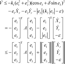
where λ_min(A) denotes the minimum eigenvalue of matrix A. Therefore, the stability of the error dynamic equation and tracking with bounded error are guaranteed outside the detection region. Moreover, we can decrease the tracking error by increasing the gains k₁ and k₂.

2. When the robot is inside the detection range (l < d_ro < L), Assumption 2 implies Ẋ_r = Ẏ_r = 0, the inequality(46) becomes:

\begin{array}{l} \dot{V} \leq - k_{1} {(\cos e_{3} + δ \sin e_{3})}^{2} (E_{X}^{2} + E_{Y}^{2}) \\ - | e_{3} | (k_{2} | e_{3} | - ε) \\ \leq - | e_{3} | (k_{2} | e_{3} | - ε) \end{array}

(50)

V̇ is negatively defined for:

| e_{3} | > \frac{ε}{k_{2}}

(51)

Hence, as shown by Stipanovic et al. [20], since dV / dt is negatively defined V is non-increasing inside the detection region. Since:

\lim_{‖ z - z_{o} ‖ \to l^{+}} V_{o b} = \infty

(52)

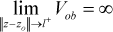
where z = [X Y]^T and z_o = [X_o Y_o]^T obstacle avoidance is guaranteed.

Remark 4. The singularity condition E_X = E_Y = 0 can occur in the following two cases: The first case occurs outside the detection region where:

\frac{\partial V_{o b}}{\partial X} = \frac{\partial V_{o b}}{\partial Y} = 0

which corresponds to e₁ = e₂ = 0 and this case can easily be handled using zero controllers u = v = 0. The second case occurs inside the detection region where the condition corresponds to a singularity in which the reference direction vector for tracking is of opposite but equal magnitude to the direction vector for avoiding collision; this results in a deadlock situation. This case can be handled by changing the reference trajectory to drive the robot out of the singularity. We do not investigate this case further in this paper.

5. Simulation results

To validate the effectiveness of the proposed adaptive control scheme, we perform simulations for trajectory tracking and obstacle avoidance for mobile robots in the presence unknown sliding. In this simulation we choose the system parameters as r = 0.125m and b=0.5m. The detection and avoidance radii are L = 4m and l = 2m.

5.1 Straight line reference trajectory tracking

In this case, a straight line reference trajectory is considered. The equation of the straight line reference trajectory is given as ${\begin{matrix} X_{r} = t \\ Y_{r} = t \end{matrix}$ , where 0s ≤ t ≤ 40s is the simulation time. The reference velocities v_r and w_r are chosen as v_r = 2m/s and ω_r = 0rad/s. The obstacle is located at (X_o, Y_o) = (8m, 10m). The initial postures of the reference robot and the actual robot are set at $[X_{r} (0), Y_{r} (0), θ_{r} (0)] = [0m, 0 m, \frac{π}{4} rad]$ and $[X (0), Y (0), θ (0)] = [- 2 m, - 2 m, \frac{π}{4} rad]$ respectively.

First, we assume that the wheels' sliding described by [i_L, i_R,δ]=[0.15,-0.15,0.1sin(0.2t)] only in fluences the mobile robot after t = 8. The controller and sliding model observer gains are chosen as L₁ = |ẋ sin θ|, L₂ = 0.3, L₃ =4r/bω_L and L₄ =4r/bω_R. The parameters of the low pass filter are chosen as γ₁ = 30, γ₂ = 20 and γ₃ = 50. The tracking and obstacle avoidance results of the proposed control system are shown in Fig.5. Fig. 5a reveals that the proposed adaptive control system can overcome the effect of sliding while obstacle avoidance is guaranteed. Tracking errors of the proposed control system are shown in Figs. 5b∼5d, we can observe in Figs. 5b∼5d that the tracking errors converge asymptotically to zero except in the range that the mobile robot detects the obstacle because the sliding effect is considered. In addition, the distance between the robot and obstacle is shown in Fig. 5e. In this figure, notice that this distance is always larger than the avoidance radius l = 2m, namely there is no collision between the robot and the obstacle. Meanwhile, it can be seen from Fig.5 f∼h, the siding parameters can be estimated precisely by the SMO.

Figure 5.

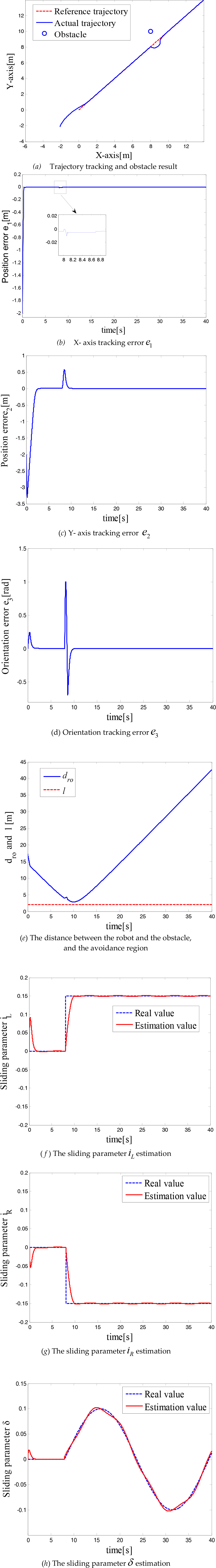
simulation results for a straight line reference trajectory in the presence of wheel's sliding

From Fig.5, we can see that the proposed control method can effectively overcome the wheels' sliding for the straight line trajectory tracking and obstacle avoidance of mobile robots.

5.2 The curved line reference trajectory tracking

In this case, we consider a curved line reference trajectory generated by reference velocities v_r = 2m/s and ω_r = 0.2rad/s for 0 ≤ t ≤ 40. The equation of the straight line reference trajectory is given as: ${\begin{matrix} X_{r} = 10 \cos (0.2 t) \\ Y_{r} = 10 \sin (0.2 t) \end{matrix}$

In addition, it is assumed that the obstacle is located at (X_o, Y_o) = (-7,-0.5). The initial positions of the reference trajectory and the actual mobile robot are chosen as ${[X_{r} (0), Y_{r} (0), θ_{r} (0)]}^{T} = {[10m, 0 m, \frac{π}{4} rad]}^{T}$ and ${[X (0), Y (0), θ (0)]}^{T} = {[7 m, 0 m, \frac{π}{4} rad]}^{T}$ respectively.

The wheels' sliding is described by:

[i_L,i_R,δ] = [0.15,-0.15, 0.6cos(0.2t)] and influences the mobile robot after t = 15.

To simplify the complexity of the simulation, the control system parameters, control parameters and the parameters of the low pass filter are all the same as in the previous simulation.

Figure 6.

Simulation results for a curved line reference trajectory in the presence of the wheels' sliding

The simulation results are shown in Fig. 6, where the proposed adaptive control system can compensate for the sliding effects and has good performance in obstacle avoidance (see Fig. 6a∼d). In addition, Fig. 6e reveals that there is no collision between the robot and the obstacles. Fig.6 f∼h show the three sliding parameters can be estimated accurately in real time by the SMO.

From Fig.6, we draw a conclusion that the proposed control approach has good tracking and obstacle avoidance performance for the curved path regardless of the effects of the unknown sliding.

Further, from Fig.5 and Fig.6, we discover that the proposed control method can avoid obstacles and overcome effectively the sliding influence for the given path tracking of mobile robots. This is mainly because the designed tracking control laws (equations (37) and (38)) have adaptive abilities and whose sliding parameters are adaptively modifying. What's more, when a robot's sliding parameters change, the tracking controller can automatically adjust these parameters to meet the demands of the mobile robot in the real environment by the sliding model observer. Even if the system sliding parameters i_L, i_R and δ change abruptly, the sliding model observer can still estimate sliding parameters rather accurately. Consequently, the adaptive tracking control algorithm has good robustness and the adaptive ability to face sliding parameter perturbations of the mobile robot.

6. Conclusions

We have presented an approach to design an adaptive controller for the tracking and obstacle avoidance of mobile robots in the presence of the wheels' unknown sliding at the kinematic level. The robot kinematic model has been induced from the model in the absence of sliding. A novel adaptive control system for mobile robots has been designed using the Lypunov design technique. Meanwhile, a sliding model observer is used to estimate sliding parameters online. We have proved its stability and have induced the control laws to compensate for unknown sliding from Lyapunov stability approach with the potential function. Finally, simulation results have shown the proposed controller has good tracking and obstacle avoidance performance and robustness against the unknown wheel sliding.

Footnotes

7. Acknowledgments

This work is supported in part by the Chongqing Natural Science Foundation (No. CSTC2012JJB40002), the Chongqing Science and Technology Grant funded by the Chongqing Government (No. CSTC, 2011AB2052) and the National High Technology Research and Development Program of China (No. 2006AA04A124).

References

Jiang

Z.P.

Nijmeijer

“Tracking control of mobile robots: A case study in backstepping”, Automatica, Vol. 33, No.7, pp. 1393–1399, 1997.

Fukao

Nakagawa

Adachi

“Adaptive tracking control of a nonholonomic mobile robot”, IEEE Transactions on Robotics and Automation, Vol. 16, No.5, pp. 609–615, 2000.

Dixon

W.E.

Queiroz

M.S.

Dawson

D.M.

Flynn

T.J.

“Adaptive tracking and regulation of a wheeled mobile robot with controller/ update law modularity”, IEEE Transactions on Control Systems Technology, Vol. 12, No.1, pp. 138–147, 2004.

Dong

Kuhnert

K. D.

“Robust adaptive control of nonholonomic mobile robot with parameter and nonparameter uncertainties”, IEEE Transactions on Robotics, Vol. 21, No.2, pp. 261–266, 2005.

K.D.

Jiang

Z.P.

Pan

“Simultaneous tracking and stabilization of mobile robots: An adaptive approach”, IEEE Transactions on Automatic Control, Vol.49, No.7, pp. 1147–1152, 2004.

Dong

Huo

Tso

S.K.

W.L.

“Tracking control of uncertain dynamic nonholonomic system and its application to wheeled mobile robots”, IEEE Transactions on Robotics and Automation, Vol. 16, No. 6, pp. 870–874, 2000.

Lee

T.C.

Song

K.T.

Lee

C.H.

Teng

C.C.

“Tracking control of unicycle-modeled mobile robots using a saturation feedback controller”, IEEE Transactions on Control Systems Technology, Vol. 9, No. 2, pp. 305–318, 2001.

Sousa

C.D.

Hemerly

E.M.

Galvao

R.K.H.

“Adaptive control for mobile robot using wavelet networks”, IEEE Transactions on Systems, Man and Cybernetics, Vol. 32, No.4, pp. 493–504, 2002.

Fierro

Lewis

F. L.

“Control of a nonholonomic mobile robot using neural networks”, IEEE Transactions on Neural Networks, Vol. 9, No. 4, pp. 589–600, 1998.

10.

Yoo

S.J.

Choi

Y.H.

Park

J. B.

“Generalized predictive control based on self-recurrent wavelet neural network for stable path tracking of mobile robots: Adaptive learning rates approach”, IEEE Transactions on Circuits and Systems I Regular Paper, Vol. 53, No. 6, pp. 1381–1394, 2006.

11.

Park

Yoo

S.J.

Choi

Y.H.

Park

J.B.

“A simple adaptive control approach for trajectory tracking of nonholonomic electrically driven mobile robots”, IEEE Transactions on Control Systems Technology, Vol. 18, No. 5, pp. 1199–1206, 2010.

12.

Castillo

Martinez-Marroquin

Melin

Valdez

Soria

“Comparative study of bio-inspired algorithms applied to the optimization of type-1 and type-2 fuzzy controllers for an autonomous mobile robot”, Information Sciences, Vol. 192, No. 6, pp. 19–38, 2012.

13.

Melendez

Castillo

Garza

A. A.

“A Fuzzy Reactive Controller of a Mobile Robot”, Soft Computing for Intelligent Control and Mobile Robotics, Vol. 318, pp. 225–232, 2011.

14.

Martínez-Soto

Castillo

Aguilar

L. T.

“Optimization of interval type-2 fuzzy logic controllers for a perturbed autonomous wheeled mobile robot using genetic algorithms”, Information Sciences, Vol. 179, No. 13, pp. 2158–2174, 2009.

15.

Corradini

M.L.

Leo

Orlando

“Robust stabilization of a mobile robot violating the nonholonomic constraint via quasi-sliding modes”. Proceeding of American Control Conference, pp. 3935–3939, 1999.

16.

Wang

Z. P.

S. S.

Lee

T. H.

“Adaptive neural network control of a wheeled mobile robot violating the pure nonholonomic constraint”, Proc. IEEE Int. Conf. Decision and Control, pp. 5198–5203, 2004.

17.

Wang

Low

C. B.

“Modeling and analysis of skidding and slipping in wheeled mobile robots: Control design perspective”, IEEE Transactions on Robotics, Vol. 24, No. 3, pp. 676–687, 2008.

18.

Low

C.B.

Wang

“GPS-based path following control for a car-like wheeled mobile robot with skidding and slipping”, IEEE Transactions on Control Systems Technology, Vol. 16, No. 2, pp. 340–347, 2008.

19.

Low

C.B.

Wang

“GPS-based tracking control for a car-like wheeled mobile robot with skidding and slipping”, IEEE Transactions on Mechatronics, Vol. 13, No. 4, pp. 480–484, 2008.

20.

Stipanovic

D. M.

Hokayem

P. F.

Spong

M. W.

and Šiljak

D. D.

“Cooperative Avoidance Control for Multiagent Systems”. Journal of Dynamic Systems, Measurement and Control, Vol.129, No.5, pp. 699–707, 2007.

21.

Dong

“Tracking Control of Multiple-Wheeled Mobile Robots With Limited Information of a Desired Trajectory”, IEEE Transactions on Robotics, VOL. 28, NO. 1, pp. 262–268, 2012.

22.

K. D.

“Formation tracking control of unicycle-type mobile robots”, IEEE Transactions on Control Systems Technology, Vol. 16, No. 3, pp. 527–538, 2008.

23.

Yoo

S. J.

“Adaptive tracking control for a class of wheeled mobile robots with unknown skidding and slipping”. IET Control Theory and Applications, Vol.4, No. 10, pp. 2109–2119, 2010.

24.

Yoo

S. J.

“Adaptive tracking and obstacle avoidance for a class mobile robots in the presence of unknown skidding and slipping”, IET Control Theory and Applications, Vol.5, No. 14, pp. 1597–1608, 2011.

25.

Zhou

Jianda

Han

Xianzhong

Dai

Backstepping based global exponential stabilization of a tracked mobile robot with slipping perturbation. Journal of bionic engineering, Vol. 8, No.1, pp. 69–76, 2011.

26.

Utkin

Guldner

and Shi

“Sliding Mode Control in Electromechanical Systems,” Taylor & Francis Inc., 325 Chestnut Street, Philadelphia, Pennsylvania, 1999.

27.

Edwards

and Spurgeon

S. K.

“Sliding mode control: Theory and applications”, London; Taylor & Francis, 1998.

28.

Stotsky

and Hu

“Control of Car-like Robots using Sliding Observers for Steering Angle Estimation,”

Proceeding of the 36th Conference on Decision & Control, San Diego, California USA. December, 1997.

29.

McCann

R. A.

Islam

M. S.

and Hussain

, “Application of sliding-mode observer for position and speed estimation in switched reluctance motor drives”, IEEE Transactions on Industry Applications, Vol. 37, No. 1, pp. 51–58, 2001.

30.

Mboup

Join

Fliess

“Numerical differentiation with annihilators in noisy environment”, Numerical Algorithms, Vol. 50, No. 4, pp. 439–467, 2009.

Adaptive Tracking and Obstacle Avoidance Control for Mobile Robots with Unknown Sliding

Abstract

Keywords

1. Introduction

2. Kinematic model of a wheeled mobile robot in the presence of sliding

3. Robot sliding parameter estimation schemes

3.1 Design of nonlinear sliding model observer

3.2 Determination of switching gains

4. Design of the tracking and obstacle avoidance controller

4.1 Potential function for obstacle avoidance

4.2 Design of controller

4.2.1 Control objective

4.2.2 Design of controller

4.2.3 Stability analysis of control system

5. Simulation results

5.1 Straight line reference trajectory tracking

5.2 The curved line reference trajectory tracking

6. Conclusions

Footnotes

7. Acknowledgments

References