Sage Journals: Discover world-class research

Abstract

Visual servoing has been around for decades, but time delay is still one of the most troublesome problems to achieve target tracking. To circumvent the problem, in this paper, the Kalman filter is employed to estimate the future position of the object. In order to introduce the Kalman filter, accurate time delays, which include the processing lag and the motion lag, need to be obtained. Thus, the delays of the visual control servoing systems are discussed and a generic timing model for the system is provided. Then, we present a current statistical model for a moving target. A fuzzy adaptive Kalman filter, which is evolved from the Kalman filter, is introduced based on the current statistical model. Finally, a two DOF visual controller based variable structure control law for micro-manipulation is presented. The results show that the proposed adaptive Kalman filter can improve the ability to track moving targets.

Keywords

Timing Model Kalman Filter Visual Servoing Target Tracking Micro Manipulation

1. Introduction

In the past ten years, microscopic visual servoing systems have been used widely in micromanipulator control for catching a target and mounting a part. When the object to be manipulated is controlled, which means that the object is static or the trajectory of the object is known, visual servoing control is easily achieved. Papanikolopoulos [1] presented algorithms to allow an eye-in-hand manipulator to track unknown-shaped 3-D objects moving in two-dimensional (2-D) space. The object's trajectory was either a line or an arc. Hashimoto [2] proposed a visual feedback control strategy for an eye-in-hand manipulator to follow a circular trajectory. However, when the object can't be controlled, i.e., the object's trajectory is uncertain, the visual servoing system often performs poorly due to the low sampling rate of the cameras and the time delays, which are created by image processing and motion control. A lot of similar problems have been discussed in the literature [3 -5]. From the above systems, we notice that the motion of the object was smooth and limited to a known class of trajectories.

In this paper, we seek to extend this to let the robot follow a completely unknown trajectory.

There are two difficulties to be tackled in the task of tracking a moving object with a microscopic visual servoing system [6, 7]. The main difficulty is the delays, which include two parts: the processing lag and the motion lag. The processing lag is introduced by the time needed to acquire and process the image, while the motion lag is produced because the slow rate of update for visual feedback results in larger-than-desired motions between updates. The second difficulty is that the maximum possible rate for visual sensing and processing is much slower than the minimum required rate for mechanical control. A common approach to overcome these problems, especially the time delays, is to introduce predictive algorithms, such as the Kalman filter [7].

The Kalman filter is well known for its use in optimal estimation and is especially suitable for a system with disturbances and measurement errors [8]. The traditional Kalman filter formulation assumes complete a priori knowledge of the process noise covariance matrix Q(k) and the measurement noise covariance matrix R(k). However, in most practical applications, these matrices are initially estimated or, in fact, are unknown. The problem here is that the optimality of the estimation algorithm in the Kalman filter setting is closely connected to the quality of these a priori noise matrices. It has been shown how poor estimates of the input noise matrices may seriously degrade Kalman filter performance and even provoke divergence of the filter [9]. Calculation of matrix R(k) for a particular measurement system is a straight-forward process. But obtaining the matrix Q(k) involves extensive experimentation and complex mathematical analysis. It is also not guaranteed that the matrices Q(k) and R(k) remain constant with time in highly non-stationary noise conditions. Thus, it is imperative to continuously tune the Kalman filter accounting for the changing noise conditions in order to get good filter performance.

Many adaptation schemes for tuning the Kalman filter were previously developed, following both conventional adaptation [10] and Fuzzy Logic adaptation [11]. Moghaddamjoo and Kirlin propose a method to adapt the Kalman filter to changes in the input forcing functions and the noise statistics [12]. Mohamed and Schwarz propose an adaptive Kalman filter which shows a major improvement over the conventional one through the adaptation of R(k)/Q(k) [13]. The performance of the adaptive Kalman filter, for most of the navigation parameters used, is improved by almost 50% or more when compared to that of the conventional filter. The main advantage of the adaptive technique is its weaker reliance on a priori statistical information. The combination of fuzzy logic and the Kalman filter is not new. Some researchers [14, 15] present probabilistic Kalman filters for mobile robots, where fuzzy rules are used to adapt R(k)/Q(k). Escamilla-Ambrosio and Mort presented a fuzzy inference system to adapt the measurement noise covariance matrix R(k) or the process noise covariance matrix Q(k) of a Kalman filter [16]. It was observed that better performance was obtained with the fuzzy adaptive Kalman filter than that obtained with both a Kalman filter without adaptation and a traditional adaptive Kalman filter.

In this paper, we introduce a novel adaptive Kalman filter. Based on the current statistical model, we propose a developed adaptive Kalman algorithm, which estimates the process noise covariance matrix Q(k) by a new formula (10). Then, an improved fuzzy adaptive Kalman filter is applied to estimate the covariance matrix R(k) and eliminate the influence of the history data. The experimental results show that the improved fuzzy Kalman filter can reduce prediction error and sense the variation of motion faster. The results are compared with those obtained using a conventional Kalman filter and a traditional fuzzy Kalman filter [16]. The improved fuzzy adaptive Kalman filter shows better results than its traditional counterparts.

The main task of the algorithm is to predict the position of the object in the next period of the image. For achieving this goal, we should first know accurately the delay time of the visual servoing system. So, a generic timing model for the visual servoing system is proposed to get the accurate delay time [6]. In order to describe the target motion, a current statistical model is presented [17 -19]. In the current statistical model, the target's acceleration is characterized by a modified Rayleigh probability density function and time-correlated by its mean value. Thus, the current statistical model can detect the target manoeuvre accurately and quickly.

To meet the demands of a high-precision tracking task, the visual servoing method is employed to guide the end effectors towards the moving object. Since the system's precise calibration is complicated and difficult, especially for micro-manipulation, we use the uncalibrated method to estimate the image Jacobian matrix online [20]. Then, a variable structure controller [21, 22] is applied to our micro manipulation system to track a moving object. The variable structure control is robust to parameter uncertainty and external disturbance because of the sliding motion on a predefined hyper plane. The experiments of visual servoing with the improved fuzzy Kalman filter in microscopes confirm that the proposed method is effective and feasible.

This paper is organized as follows: In Section 2 we introduce our generic timing model. Section 3 describes a current statistical model to express the motion of the object. In Section 4 an improved fuzzy adaptive Kalman filter is introduced. In Section 5 visual servoing based on the fuzzy adaptive Kalman filter by using a variable structure controller is detailed. Experimental results on the performance of the proposed method are illustrated in Section 6 followed by the conclusion in Section 7.

2. Generic Timing Model

The time delay in visual servoing systems includes two parts [6]: processing lag and motion lag. The processing lag is introduced by the time required for visual sensing and processing between when the object state in reality is sensed and when the visual understanding of that object state (e.g., image tracking result) is available. The motion lag is produced by the slow rate of update for visual feedback results in larger-than-desired motions between updates when the mechanical system has completed the desired motion. It is worth noting that the maximum possible rate for complex visual sensing and processing is much slower than the minimum required rate for mechanical control.

The first step of visual servoing is visual sensing and processing. There are four main configurations for visual sensing and processing, which are serial, on-the-fly, parallel and pipeline processing. Fig. 1 shows the four cases, where t_ac presents the visual sensing time, t_p presents the visual processing time.

Figure 1.

Four main configurations of visual servo system

According to Fig. 1, on-the-fly processing has the shortest delay time, but t_ac is usually smaller than t_p in the actual system. Compared to the other three architectures, parallel processing is efficient and doesn't increase the complexity of the system. Hence, we employ parallel processing to construct the timing model. Fig. 2 depicts the proposed timing model.

Figure 2.

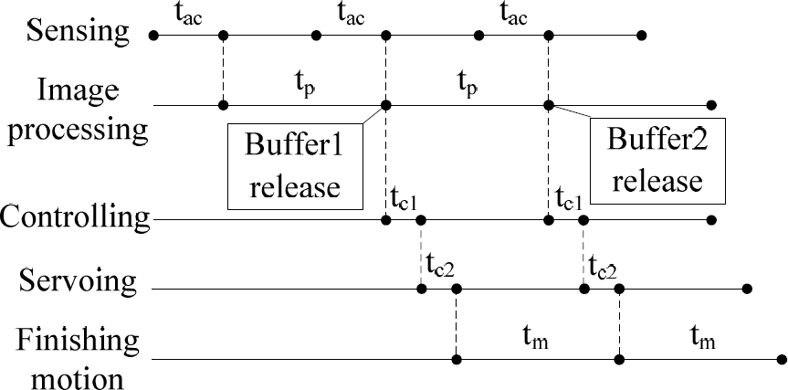
Timing model of visual servo system

There are two input buffers (commonly called “double buffering”). In this case, a second image buffer is being filled while the image data in the first buffer is being processed. Double buffering increases the throughput. In Fig. 2, t_ac presents the image acquisition time, t_p presents the image processing time, t_c1 presents the time that the visual controller outputs the control signal, t_c2 presents the servoing time of the robot joint and t_m presents the time that the manipulator takes to move from the current position to the desire position.

According to Figure 2, the precise delay time T is:

T = t_{ac} + t_{p} + t_{c1} + t_{c2} + t_{m} .

(1)

3. Improved Adaptive Kalman Filter Based on the Current Statistical Model

3.1 Current Statistical Model

Based on the timing model, the current statistical model is introduced to describe the motion of the target. The current statistical model is a Singer model modified to have non-zero mean, time-correlated acceleration [19]. It is assumed that the acceleration of the target a(t) is satisfied with the equation as following:

a (t) = \hat{a} (t) + \bar{a} (t)

(2)

Where â(t) is a zero-mean Markov process, ā(t) is the mean of acceleration, assumed to be constant in every sampling period.

The current statistical model based on the visual servo system is:

\begin{array}{l} X (k) = Φ (k) X (k - 1) + U (k) \bar{a} + W (k) \\ Z (k) = H (k) X (k) + V (k) \end{array}

(3)

With

Φ (k) = (\begin{matrix} 1 & T & \frac{1}{α^{2}} (α T - 1 + e^{- α T}) & 0 & 0 & 0 \\ 0 & 1 & \frac{1}{α} (1 - e^{- α T}) & 0 & 0 & 0 \\ 0 & 0 & e^{- α T} & 0 & 0 & 0 \\ 0 & 0 & 0 & 1 & T & \frac{1}{α^{2}} (α T - 1 + e^{- α T}) \\ 0 & 0 & 0 & 0 & 1 & \frac{1}{α} (1 - e^{- α T}) \\ 0 & 0 & 0 & 0 & 0 & e^{- α T} \end{matrix})

(4)

U (k) = (\begin{matrix} \frac{1}{α} (\frac{α T^{2}}{2} + \frac{1 - e^{- α T}}{α} - T) & 0 \\ T - \frac{1 - e^{- α T}}{α} & 0 \\ 1 - e^{- α T} & 0 \\ 0 & \frac{1}{α} (\frac{α T^{2}}{2} + \frac{1 - e^{- α T}}{α} - T) \\ 0 & T - \frac{1 - e^{- α T}}{α} \\ 0 & 1 - e^{- α T} \end{matrix})

(5)

H (k) = (\begin{matrix} 1 & 0 & 0 & 0 & 0 & 0 \\ 0 & 0 & 0 & 1 & 0 & 0 \end{matrix})

(6)

Where X(k) = [x ẋ ẍ y ẏ ÿ]^T, x and y are the predicted coordinates of the moving object in the next image which will need to be processed, the predictive velocity of the object in the image coordinate system is presented by ẋ and ẏ; ẍ and ÿ represent the predicted acceleration of the object in the next image, while Z(k) = [u v] ^T is the coordinate of the object that is measured in the current image; α is the acceleration correlation coefficient; V(k) is the zero-mean gauss white noise, whose variance is R(k). The process noise W(k) is a discrete time sequence of white noise and E[W(k)W^T (k + j)] = 0,(∀j ≠ 0).

Process noise covariance matrix Q(k) is given by:

Q (k) = E [W (k) W^{T} (k)] = 2 α σ_{a}^{2} (\begin{matrix} q_{11} & q_{12} & q_{13} \\ q_{12} & q_{22} & q_{23} \\ q_{13} & q_{23} & q_{33} \end{matrix})

(7)

Where:

\begin{array}{l} q_{11} = \frac{1}{2 α^{5}} (1 - e^{- 2 α T} + 2 α T + \frac{2 α^{3} T^{3}}{3} - 2 α^{2} T^{2} - 4 α T e^{- α T}) \\ q_{12} = \frac{1}{2 α^{4}} (e^{- 2 α T} + 1 + 2 e^{- α T} + 2 α T e^{- α T} - 2 α T - α^{2} T^{2}) \\ q_{13} = \frac{1}{2 α^{3}} (1 - e^{- 2 α T} - 2 α T e^{- α T}) \\ q_{22} = \frac{1}{2 α^{3}} (4 e^{- α T} - 3 - e^{- 2 α T} + 2 α T) \\ q_{23} = \frac{1}{2 α^{2}} (e^{- 2 α T} + 1 - 2 e^{- α T}) \\ q_{33} = \frac{1}{2 α} (1 - e^{- 2 α T}) \end{array}

Variance σ is the modified Rayleigh distribution variance of the manoeuvring acceleration:

\begin{array}{l} σ_{a}^{2} = \frac{4 - π}{π} {[a_{max} - \hat{a} (t)]}^{2}, \hat{a} (t) > 0 \\ σ_{a}^{2} = \frac{4 - π}{π} {[a_{- max} + \hat{a} (t)]}^{2}, \hat{a} (t) < 0 \end{array}

(8)

Where a_max is the positive upper limit of the acceleration, while a_–max is the negative lower limit of the acceleration.

3.2 Improved Adaptive Kalman Filter

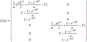
For any model of the form (3), the prediction X(k | k – 1) of the signal X(k) given measurements of X(0),…, X(k – 1) can be calculated using a Kalman filter [23]. In more detail, we have

\begin{array}{l} \hat{X} (k | k) = \hat{X} (k | k - 1) + K (k) [Z (k) - H (k) \hat{X} (k | k - 1)] \end{array}

(9.1)

\begin{array}{l} \hat{X} (k | k - 1) = Φ (k) \hat{X} (k - 1 | k - 1) + U (k) \bar{a} (k) \end{array}

(9.2)

\begin{array}{l} P (k | k - 1) = Φ (k) P (k - 1 | k - 1) Φ^{T} (k) + Q (k - 1) \end{array}

(9.3)

K (k) - P (k | k - 1) H^{T} (k) {[H (k) P (k | k - 1) H^{T} (k) + R (k)]}^{- 1}

(9.4)

\begin{array}{l} P (k | k) = [I - K (k) H (k)] P (k | k - 1) \end{array}

(9.5)

Where X̂(k – 1 | k – 1) is a prediction of the hidden model state, P(k | k – 1) is the predicted covariance matrix of the state and K(k) is called the Kalman filter gain. Looking at the above formulae in more detail, we can see how process noise V(k) and measurement noise W(k) influence the predicted covariance matrix P(k | k – 1).

We regard [ẍ(k | k – 1) ÿ(k | k – 1)] ^T , which is the prediction of [ẍ(k) ÿ(k)] ^T , as ā(k), i.e., the mean of acceleration. Then, we fulfil the Kalman algorithm.

The algorithm mentioned above is very much affected by a_max and a_–max. If the absolute values of a_max and a_–max are small, the tracking accuracy is high, but the system is slow to respond when the tracking target's motion changes tremendously. If the absolute values of a_max and a_–max are large, the system has a quick response with lower tracking accuracy. To cover this defect, we introduce a developed adaptive Kalman algorithm [24]. Let:

σ_{α}^{2} = \frac{2 [\hat{x} (k | k) - \hat{x} (k | k - 1)]}{T^{2}}

(10)

4. Improved Fuzzy Adaptive Kalman Filter

4.1 Estimate the Covariance matrices R(k)

In this section, a fuzzy adaptive Kalman filter is applied to estimate the covariance matrices R(k). Fuzzy control is one of the useful control paradigms for uncertain and ill-defined nonlinear systems. Control actions of a fuzzy controller are described by some linguistic rules. We adjust R(k) by monitoring the innovation sequence {ε(i),i = 1,.., k}, which is defined as:

ε (i) = Z (i) - \hat{Z} (i)

(11)

where Z(i) is the real measurement and ẑ(i) is the predicted value of Z(i). The innovation sequence represents the information of the new observation and is considered the most relevant source of information for filter adaptation. In theory, the innovation sequence is a zero mean gauss white noise sequence:

E [ε (k)] = 0

(12)

The theoretical covariance matrix {ε(i), i = 1,…, k} can be derived from the Kalman filter:

P [ε (k)] = H (k) P (k | k - 1) H^{T} (k) + R (k)

(13)

However, in practice, the innovation sequence is affected by model uncertainty and noise statistical uncertainty. We use [25]′s method to obtain the equalizing value and covariance matrix of the innovation sequence:

\begin{array}{l} E^{'} [ε (k)] = \frac{1}{N} \sum_{i = k - N + 1}^{k} ε (i) \\ P^{'} [ε (k)] = \frac{1}{N} \sum_{i = k - N + 1}^{k} ε (i) ε^{T} (i) \end{array}

(14)

N is chosen empirically to give some statistical smoothing. Then, we get the error formula between the theoretical covariance matrix and the practical covariance matrix of the innovation sequence:

\begin{array}{l} Δ P^{'} [ε (k)] = P [ε (k)] - P^{'} [ε (k)] \\ = H (k) P (k | k - 1) H^{T} (k) + R (k) - \frac{1}{N} \sum_{i = k - N + 1}^{k} ε (i) \end{array}

(15)

Notice thatE' and ΔP', whose values should be zero in an optimal situation, reflect the state of the current Kalman filter. When the values of E′ and ΔP′ are not zero, this indicates that the predicted value of Z(k) is not correct. Then, we can adjust R(k) to let the Kalman filter tend towards stability. The adjustment rules of R(k) are as follows:

(1)

If E′ = 0 and ΔP′ = 0, R(k) should stay fixed.

(2)

If E′ > 0, increase R(k).

(3)

If E′ < 0, decrease R(k).

(4)

If ΔP′ > 0, increase R(k).

(5)

If ΔP′ < 0, decrease R(k).

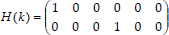
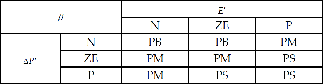
Based on the adjustment rules, E′ and ΔP′ are chosen as the input variables of the Fuzzy logical controller. The Fuzzy Kalman filter proposed here receives the values of E′ and ΔP′ at each time instant and works out a scalar value called the adjustment factor β. β indicates the amount which the measurement noise covariance matrix R(k) should be scaled by in order to compensate for the varying noise disturbances. The new measurement noise covariance at each time instant is calculated as:

\hat{R} (k) = β R (k)

(16)

The range of β is [0.8 1.2], while the range of E′ is [-0.5 0.5] and the range of ΔP′ is selected as [-10 10].

The input variables are E′ and ΔP′ while their membership functions are N: Negative, ZE: Zero, P: Positive. The membership functions of the output variable of the controller are PS: Positive Small, PM: Positive Medium and PB: Positive Big. We use triangular membership functions of the fuzzy sets defined in the input spaces. The output linguistic variables are represented using a trapezoidal membership function; see Fig. 3. The collection of the rules is shown in Table 1.

Table 1.

Fuzzy rules of the fuzzy Kalman filter

β		E′
β		N	ZE	P
ΔP'	N	PB	PB	PM
	ZE	PM	PM	PS
	P	PM	PS	PS

Figure 3.

The membership functions of E′, ΔP and β

4.2 Improved Fuzzy Adaptive Kalman Filter

From (9.1) we know that X̂(k | k) does not really provide completely new information because some of the information is obtained by predictions from previous filter states, which contain all the predicted information from X(0) to X(k – 1). If the object's motion is changed, the old data can't reflect the current motion of the object. When the motion changes abruptly, the Kalman filter can't follow the variation in time, due to the influence of the history data. The variation of the motion can be monitored by the innovation sequence. In order to let the Kalman filter sense the variation of the motion faster, we adjust P(k | k – 1) in (9.3) according to the variation of the innovation sequence by the fuzzy controller. We rewrite (9.3) as follow:

\hat{P} (k | k - 1) = γ \times Φ (k) P (k - 1 | k - 1) Φ^{T} (k) + Q (k - 1)

(17)

We calculate the error between the current equalizing value and the last equalizing value of the innovation sequence as follow:

Δ E^{'} [ε (k)] = | E^{'} [ε (k)] - E^{'} [ε (k - N)] |

(18)

where E'[ε(k)] is the current equalizing value of the innovation sequence and E'[ε(k – N)] is the last equalizing value of the innovation sequence. If ΔE'[ε(k)] increases considerably, it indicates a change of the motion of the object. The adjustment rules of P(k | k – 1) are as follows: (1)

If ΔE[ε(k)] > E'[ε(k – N)], increase γ.

(2)

If ΔE[ε(k)] < E'[ε(k – N)], γ = 1.

According to the adjustment rules, if the value of ΔE[ε(k)] is greater than the last equalizing value of the innovation sequence, P̂(k | k – 1) will be greater than the original value of P(k | k – 1). Hence, the influence of the innovation sequence in (9.2) will increase. X̂(k | k) can reflect the current motion more factually.

The fuzzy Kalman filter receives the value of ΔE[ε(k)] every ten time intervals. The range of ΔE[ε(k)] is [2–50], while the range of γ is [100–1000]. The membership functions of ΔE[ε(k)] are NB: Negative Big, NS: Negative Small, ZE: Zero, PS: Positive Small, PB: Positive Big. The membership functions of the output variable γ are the same as ΔE[ε(k)]. The membership functions are shown in Fig. 4.

Figure 4.

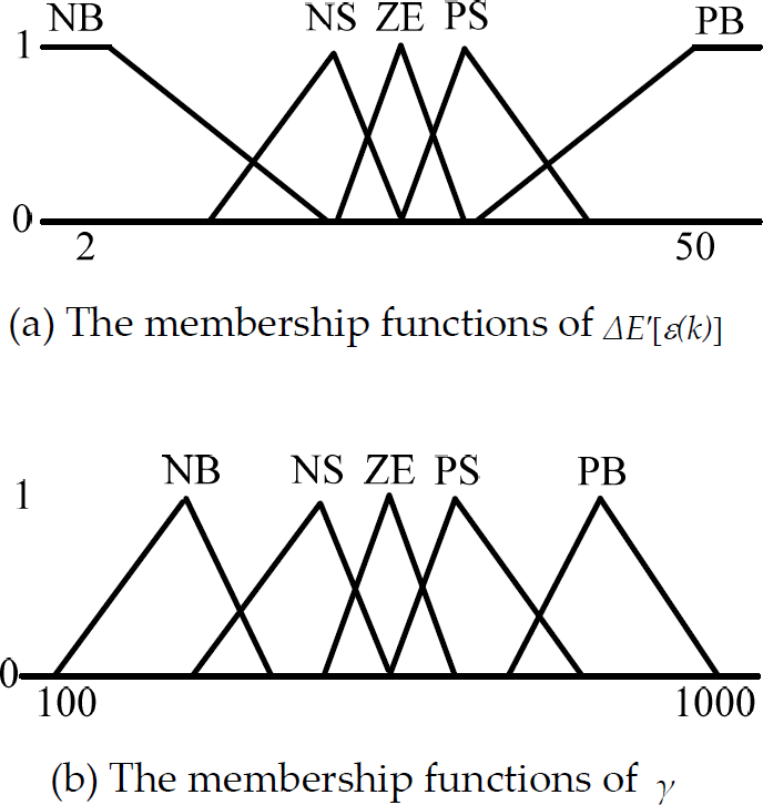
The membership functions of ΔE'[ε(k)] and γ

5. Visual Servoing Based on the Fuzzy Adaptive Kalman Filter

Visual servoing methods can be categorized into two basic groups: position-based visual servoing and image-based visual servoing (IBVS) [26]. In IBVS, a set of features is selected and fed back to the controller through an image Jacobian matrix, which represents a local, linear and differential relationship between the velocities of the image features and the joint velocities. IBVS is less sensitive to image disturbances and calibration errors compared to a position-based approach and it is inconvenient to describe tasks using image features. The position-based visual servoing needs precise calibration of the intrinsic parameters of the camera. However, system calibration is the complicated and difficult problem, especially for micro-manipulation based on microscope vision. So, our approach to visual servoing is the uncalibrated image-based one. For IBVS, the first task is to identify multi micro parts. The improved support vector machine (SVM) multi objects' identification method is used to fulfil this task [20]. The image Jacobian matrix plays a major role in IBVS. In our previous work, we used Broyden's method to estimate the image Jacobian matrix [20]. The micro manipulation tasks will be divided into horizontal (XY plane) movement and vertical (Z axis) movement. The manipulator moves in the XY plane first positioning small parts, then does so in the Z-axis, positioning small parts at the centre. Therefore, we apply two image Jacobian matrices, including a horizontal view of the image Jacobian matrix and vertical view of the image Jacobian matrix, which can complete the positioning and tracking of three-dimensional objects.

In this section, the variable structure controller is applied to our micro manipulation system to track a moving object. The variable structure control (VSC) has been widely discussed and used in various applications. The control function of VSC is designed to reach the sliding surface that is predetermined to achieve the desired performance. It is gaining importance as a universal design methodology for the robust control of linear and nonlinear systems. It offers several redeeming features from a control theory point of view [27, 28], namely, an inherent order reduction, direct incorporation of robustness against system uncertainties and disturbances and an implicit stability proof. In recent years, due to its robustness, the application of VSC on dynamic systems subject to external disturbances has been extensively studied. Many desirable properties of VSC systems are well documented [21, 22]. According to the results of previous studies on sliding surface design approaches, the performances of the controlled systems were satisfactory. Li and Xie propose a visual servoing tracking controller based on the sliding mode control theory, which exploits the epipolar geometry between a current image and a target one without requiring any a priori knowledge of the scene or precise camera calibration due to the intrinsic robustness of the control law against matched uncertainties and disturbances [29]. Simulation results showed that the control scheme can achieve good tracking performance and has strong robustness against parameter variations and external disturbances. Hence, we will focus here on a variable structure control with sliding mode, which proved its potential in visual servoing system [29].

Since the micro manipulation task is divided into horizontal (XY plane) movement and vertical (Z axis) movement, we design two DOF visual controller based VSC laws for micro manipulation.

The state equation for a visual servoing system can be written as:

M (k + 1) = M (k) + T J (k) u (k)

(19)

Where M(k) = [imx(k) imy(k)] ^T is the centre of the object that is measured in the current image, J(k) is the image Jacobian matrix, T is the sampling period of the vision system and u(k) = [ẋ_T(k) ẏ_T(k)] ^T is the manipulator end-effector velocity. The control objective of the visual servoing is to control the end-effector to achieve the desired image plane coordinate, which could be constant or changing with time.

Based on the state equation, we choose the switching plane of VSC as:

S (k) = C [M (k) - M^{*} (k)] = 0

(20)

where M*(k) = [imx*(k) imy*(k)] ^T is the desired image plane coordinate. We already know that when the object is moving, the desired image plane coordinate observed at the current time will be not the same as the desired image plane coordinate which the manipulator should move to at the current time, due to the time delay of the visual servoing system. Hence, we should estimate the actual desired image plane coordinate. (20) can be rewritten as:

S (k) = C [M (k) - {\hat{M}}^{*} (k)] = 0

(21)

Where M̂*(k) is the estimated value of the actual desired image plane coordinate by using the fuzzy adaptive Kalman filter which is described in Section 4 and:

C = d i a g (c_{1}, c_{2}), c_{1} > 0, c_{2} > 0

(22)

The u(k) is characterized by the control structure defined by:

u (k) = {\begin{cases} u^{+} (k), \begin{matrix} ​ \end{matrix} for \begin{matrix} ​ \end{matrix} S (k) > 0 \\ u^{-} (k), \begin{matrix} ​ \end{matrix} for \begin{matrix} ​ \end{matrix} S (k) < 0 \end{cases}

(23)

According to VSC, when the sliding mode occurs, Ṡ(k) should be zero, so we have:

\dot{S} (k) = C \dot{M} (k) = C J (k) u (k) = 0

(24)

We choose:

\dot{S} (k) = - W S (k) - K sgn [S (k)]

(25)

Where:

W = d i a g (w_{1}, w_{2}), w_{1} > 0, w_{2} > 0

(26)

and:

K = d i a g (k_{1}, k_{2}), k_{1} > 0, k_{2} > 0

(27)

Substituting (25) into (24), we have:

C J (k) u (k) = - W S (k) - K sgn [S (k)]

(28)

So the control law of VSC u(k) is:

u (k) = - p i n v [J (k)] C^{- 1} {W S (k) + K sgn [S (k)]}

(29)

In Eq. 29, the coefficient of S(k), which is C⁻¹W, affects the dynamic property of the visual servoing system. If the value of C⁻¹W is large, the tracking error can be eliminated as quickly as possible. When the end-effector is far from the moving target at the beginning of the visual servoing, this will cause excessive velocity and displacement of the end-effector. If the value of C⁻¹W is small, the tracking error can be reduced smoothly. However, the final tracking error is large. Hence, at the beginning of the visual servoing, the value of C⁻¹W should be small. When the end-effector moves close to the target, we should increase the value of C⁻¹W to make the tracking error as small as possible.

6. Experimental Results

6.1 Simulation

Based on the current statistical model identified in Section 3, we firstly simulate the system to evaluate the prediction performance of the Kalman filter without adaptation, the traditional fuzzy adaptive Kalman filter proposed in [16] and our improved fuzzy adaptive Kalman filter.

Three kinds of prediction task are simulated. The first task is tracking a target which is moving uniformly and in a straight line. The starting position of the target in the image coordinate system is x=0, y=0 and the velocities in the x-direction and the y-direction are both 10 mm/s. The second task is tracking a motion where the acceleration changes sharply during the movement. At the beginning, x=0, y=0. The velocities in the x-direction and the y-direction are both 20 mm/s, while the accelerations are both 1mm/s². After 14 seconds, the accelerations in the x-direction and the y-direction change to 30mm/s². The zigzag motion tracking is the third task. The beginning position of the object is x=0, y=0. The velocity in the x-direction is 1mm/s. The y-direction velocity is 10mm/s, which changes to −10mm/s after 9 seconds. The prediction error is used as a criterion to compare the different computation methods and is defined as:

E r r o r = | \hat{x} (k) - x (k) | + | \hat{y} (k) - y (k) |

(30)

Where x(k) is the real measurement and ◯(k) is the predicted value in the x-direction, y(k) is the real measurement and ŷ(k) is the predicted value in the y-direction.

The results of the simulation are shown in Fig. 5. For comparison, we show the simulation results based on the Kalman filter without adaptation, the traditional fuzzy adaptive Kalman filter proposed in [16] and our improved adaptive Kalman filter respectively.

Figure 5.

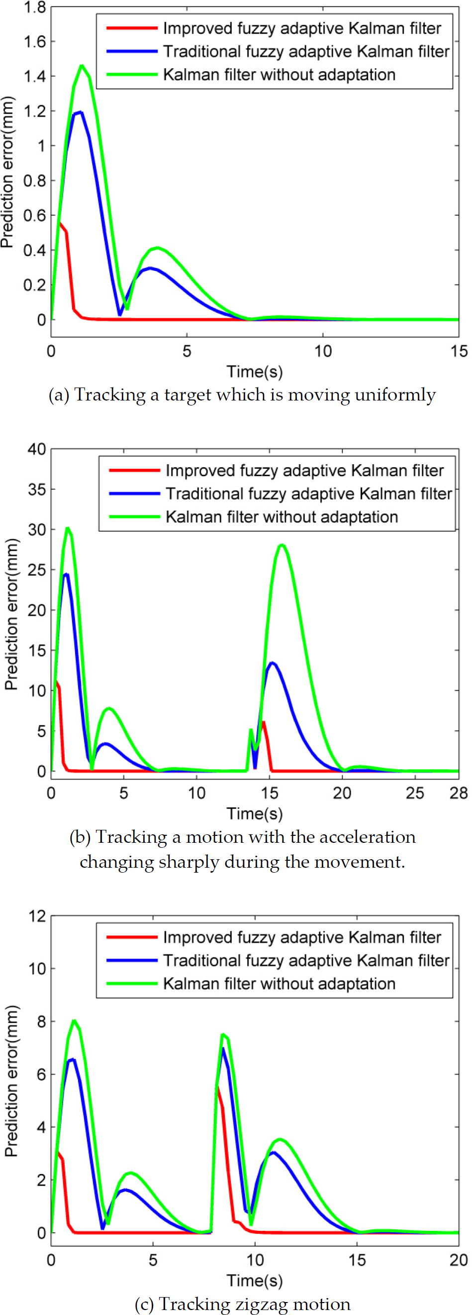
The simulation results of three tracking tasks

In Fig. 5(a), the results show that the performance of the improved fuzzy adaptive Kalman filter is better than the Kalman filter without adaptation and the traditional fuzzy adaptive Kalman filter [16]. We can get the best response and the smallest overshoot with the improved adaptive Kalman filter if the object remains in a state of uniform motion in a straight line. This effect can be observed more clearly in the Fig. 5(b) and Fig. 5(c) when the task is tracking a motion where the acceleration changed sharply during the movement and a zigzag motion. In the tracking task, if the response is poor and the overshoot is big, the camera may lose a target whose velocity or acceleration changes greatly when the tracking window is small. However, the processing time of enough large images would be too long. The improved adaptive Kalman filter can track an object with a small tracking window. It can improve system efficiency without losing the tracked object.

6.2 Visual Servoing Experiment

Object tracking is an important component of a micro visual servoing based micro assembly system [20, 30]. The system is controlled by two levels of computer control systems and consists of three parts: a micromanipulator unit, a stereo microscopic vision unit and a micro grippers unit. A triple-manipulator cooperation strategy was developed in the system to fulfil 3D micro assembly tasks. Compared with the common stereo vision configuration using two parallel views, a microscopic vision unit was developed with two perpendicular views to reduce the structural complexity of the mechanism, which includes the horizontal microscope vision and the vertical microscope vision. In the micro gripper unit, there are two kinds of micro grippers: a vacuum micro gripper and a piezoelectric (PZT) bimorph micro gripper. Fig. 6 shows the visual servoing micro manipulation system. Fig. 7 shows the original image of the operation targets and the manipulator in the microscopic environment for a vertical microscope.

Figure 6.

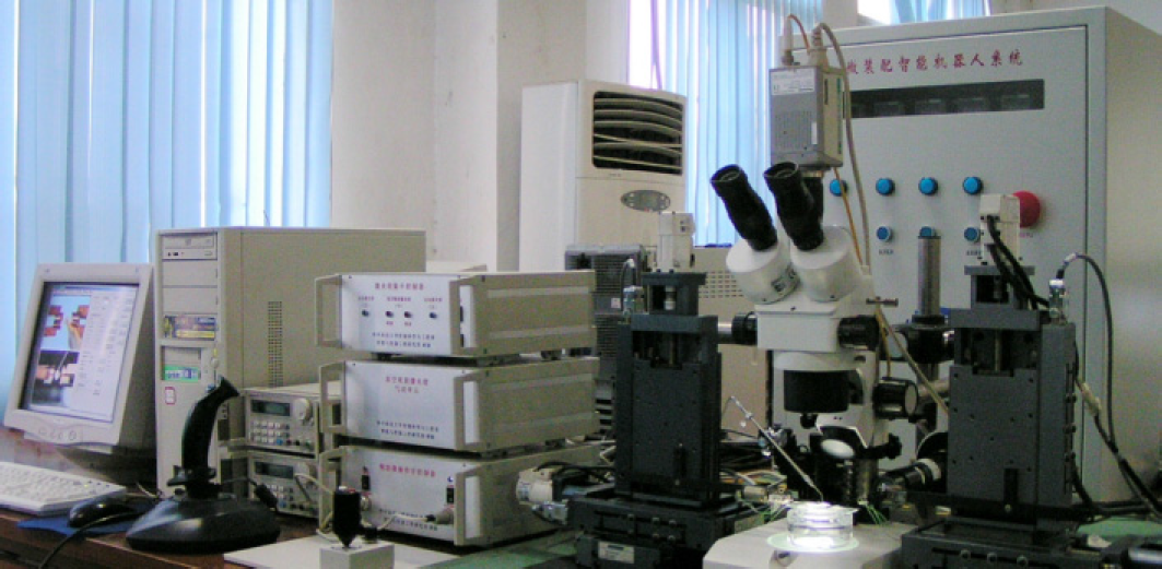
Photo of the visual servoing system

Figure 7.

The original image of the visual servoing system

In this experiment, we first attempt to predict the centre of the micro gripper in different kinds of tracking task. Fig. 8 is the image after edge extraction of the operation targets and the manipulator in the microscopic environment for a vertical microscope.

Figure 8.

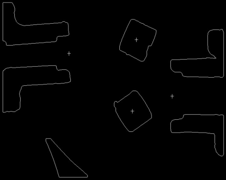
The image of the visual servoing system

The first task is predicting a micro gripper that is moving uniformly and in a straight line with a velocity of 1mm/s. The second task is predicting a micro gripper that is describing a circular motion with uniform velocity, whose radius is 20mm and angular velocity is 0.15rad/s. We use a window of 150×150 pixels to track the micro gripper, see Fig. 7. For comparison, we show the results based on the Kalman filter without adaptation, the traditional fuzzy adaptive Kalman filter proposed in [16] and our improved adaptive Kalman filter respectively. The prediction error between the centre of the manipulator and the centre of the window is shown in Fig. 9. Fig. 9(a) verifies that our improved fuzzy adaptive Kalman filter has a faster response and a smaller overshoot if the object remains in a state of uniform motion in a straight line. The final error of the improved fuzzy adaptive Kalman filter is zero. The Kalman without adaptation and the traditional fuzzy adaptive Kalman filter have the same final prediction error, which is about 1 pixel. When the micro gripper is describing a circular motion with uniform velocity, the prediction error of the improved fuzzy adaptive Kalman filter reaches a small value quickly in the first 2 seconds, however, the prediction error of the Kalman filter without adaptation and the traditional fuzzy adaptive Kalman filter remain at a large value. The final prediction error using the Kalman filter without adaptation is about 8 pixels and around 4 pixels using the traditional fuzzy adaptive Kalman filter, while the final prediction error remains at 2 pixels as time goes on using the proposed method as shown in Fig. 9(b). The results show that the proposed method has better performance.

Figure 9.

The prediction error between the centre of the manipulator and the centre of the window

In order to verify the performance of the visual servo system, two kinds of tracking tasks are studied. In the first task, we use right PZT bimorph micro gripper to track the left PZT bimorph micro gripper which is moving uniformly and in a straight line. In order to avoid collision of the two micro grippers, we set the image plane coordinate, which is the sum of a constant value and the image plane coordinate of the left PZT bimorph micro gripper, as the desired image plane coordinate at which the right PZT bimorph micro gripper should arrive.

The constant value is 300 pixels. The beginning position of left micro gripper is imx=100, imy=100. The beginning position of the desired motion is imx=100+300, imy=100. The velocity in the x-direction is 0mm/s. The y-direction velocity is 1mm/s. The tracking errors between the two PZT bimorph micro grippers are shown in Fig. 10. It is worth noting that the constant value has been subtracted in order to show the tracking errors more suitably. From Fig. 10, we can see the tracking error of y-direction error is about 5 pixels when we don't introduce the Kalman filter. The appearance of the error is caused by the time delay of the visual servoing system as we discussed in the above sections. The improved adaptive Kalman filter can eliminate the error when the end-effector is tracking an object that moves uniformly in a straight line.

Figure 10.

The tracking error for tracking the left microgripper which is moving uniformly

The second task is tracking the left PZT bimorph micro gripper that is describing a circular motion at with uniform velocity, whose radius is 20mm and angular velocity is 0.15rad/s, by using the right PZT bimorph micro gripper. The motion equation of the left PZT bimorph micro gripper is:

{\begin{cases} x = 50 \cos (0.15 t) + 100 \\ y = 50 \sin (0.15 t) + 150 \end{cases}

The starting position of left PZT bimorph micro gripper is imx=200, imy=150. The centre of the circle is (100,150). Hence, the beginning position of the desired motion is imx=200+300, imy=150. The desired centre of the circle is (400,150). The starting position of the right PZT bimorph micro gripper is imx=510, imy=160. The tracking errors between the two PZT bimorph micro grippers of the second task are shown in Fig. 11. When the left micro gripper makes a circular motion at a uniform velocity, the final tracking error in both directions is equal or less than 4 pixels when using the proposed method and the traditional fuzzy adaptive Kalman filter [16], while the tracking error fluctuates between −10 pixels and 10 pixels. However, it can be seen that the tracking error when using the traditional fuzzy adaptive Kalman filter is larger than when using the improved fuzzy adaptive Kalman filter at the beginning of the tracking task. The experimental results support the superiority of the proposed method.

Figure 11.

The tracking error for tracking the left microgripper that is describing a circular motion with uniform velocity

7. Conclusion

In this paper, we propose an improved adaptive Kalman filter for a visual servoing system to track a moving target. This method can not only track an object which moves smoothly, but also whose velocity or acceleration changes greatly. In order to introduce the improved Kalman algorithm, we establish the generic timing model of the visual servoing system and build a current statistical model which can describe the trajectory of a moving target. Based on the current statistical model, we propose a developed adaptive Kalman algorithm, which estimates the process noise covariance matrix Q(k) by an improved formula. Then, an improved fuzzy adaptive Kalman filter is applied to estimate the covariance matrices R(k) and eliminate the influence of the history data. The simulation and experimental results show that the improved fuzzy Kalman filter can reduce the prediction error and sense the variation of the motion faster. Finally, a variable structure controller is used to complete the visual servoing task of target tracking, the results show that tracking performance is improved by introducing the improved adaptive Kalman filter. The choice of parameters for the variable structure controller is important to the dynamic property of the visual servoing system. Our future work is to investigative a method which can estimate the parameters' self-adaptability.

Footnotes

8. Acknowledgments

This work is supported in parts by the National High Technology Research and Development Program 863 of China (Grant No. 2008AA8041302), the National Natural Science Foundation of China (Grant No. 60873032) and the Doctoral Program Foundation of Ministry of Education of China (Grant No. 20100142110020).

References

Papanikolopoulos

Khosla

P. K.

and Kanade

, “Visual tracking of a moving target by a camera mounted on a robot: A combination of control and vision,” IEEE Transaction on Robotics and Automation, vol. 9, no. 1, 1993, pp. 14–33.

Hashimoto

Kimoto

Ebine

and Kimura

, “Manipulator control with image-based visual servo,” in Proc. IEEE International Conference on Robotics and Automation, Scramento, CA, 1991, pp. 2267–2272.

Allen

Timcenko

Yoshimi

and Michelman

, “Automated tracking and grasping of a moving object with a robotics hand-eye system,” IEEE Transaction on Robotics and Automation, vol. 9, no. 2, 1993, pp. 152–165.

Miyazaki

Takeuchi

Matsushima

Kusano

and Hashimoto

, “Realization of the table tennis task based on virtual targets,” in Proc. IEEE International Conference on Robotics and Automation, Washington, DC, 2002, pp. 3844–3849.

Nakai

Taniguchi

Uenohara

and Yoshimi

, “A volleyball playing robot,” in Proc. IEEE International Conference on Robotics and Automation, Leuven, Belgium, 1998, pp. 1083–1089.

Liu

Hoover

A. W.

and Walker

I. D.

, “A Timing Model for Vision-Based Control of Industrial Robot Manipulators,” IEEE Transaction on Robotics, vol. 20, no. 5, 2004, pp. 891–898.

Yoon

Kosaka

and Avinash

C. K.

, “A New Kalman-Filter-Based Framework for Fast and Accurate Visual Tracking of Rigid Objects,” IEEE Transaction on Robotics, vol. 24, no. 5, 2008, pp. 1238–1251.

Durdu

O. F.

, “Fuzzy logic adaptive Kalman filtering in the control of irrigation canals,” International Journal for Numerical Methods in Fluids, vol. 64, no. 2, 2010, pp.187–208.

Escamilla-Ambrosio

P. J.

and Mort

, “A hybrid Kalman filter-fuzzy logic architecture for multisensor data fusion,” in Proc. Proceedings of the 2001 IEEE International Symposium on Intelligent Control, 2001, pp. 364–369.

10.

Gutman

and Velger

, “Tracking targets with unknown process noise variance using adaptive Kalman filtering,” in Proc. Proceeding of the 27th IEEE International Conference on Decision and Control, vol. 1, 1988, pp. 869–874J.

11.

Kobayashi

Cheok

Ka. C.

and Watanabe

, “Estimation of absolute vehicle speed using fuzzy logic rule-based Kalman filter,” in Proc. Proceeding of the American Control Conference, vol. 5, 1995, pp. 3086–3090.

12.

Moghaddamjoo

and Kirlin

L. R.

, “Robust adaptive Kalman filtering with unknown inputs,” IEEE Transactions on Acoustics, Speech and Signal Processing, vol. 37, no. 8, 1989, pp. 1166–1175.

13.

Mohamed

A. H.

and Schwarz

K. P.

, “Adaptive Kalman filtering for INS/GPS,” Journal of Geodesy, vol. 73, no. 4, 1999, pp. 193–203.

14.

Jetto

Longhi

and Venturini

, “Development and experimental validation of an adaptive extended Kalman filter for the localization of mobile robot,” IEEE Transaction on Robotics and Automation. vol. 15, no. 2, 1999, pp. 219–229.

15.

Sasiadek

J. Z.

and Wang

, “Sensor fusion based on fuzzy Kalman filtering for autonomous robot vehicle,” in Poc. Proceedings of the IEEE International Conference on Robotics and Automation, vol. 4, 1999, pp. 2970–2975.

16.

Escamilla-Ambrosio

P. J.

and Mort

, “Adaptive Kalman filtering through fuzzy logic,” in Proc. of the 7th UK Workshop on Fuzzy System, Recent Advances and Practical Applications of Fuzzy, Nero-Fuzzy and Genetic Algorithm-Based Fuzzy Systems, U.K., 2000, pp. 67–73.

17.

X. N.

Qin

Guo

R. H.

and Li

G. B.

, “A variable-structure IMM filtering algorithm based on current statistical model,” in Proc. Proceedings of the 2009 International Conference on Mechatronics and Automation, 2009, pp. 2983–2988.

18.

D. W.

Xie

W. X.

Huang

J. J.

Huang

J. X.

and Jin

K.C.

, “Current Statistical Model Based on Maximum Entropy Fuzzy Clustering,” in Proc. 10th International Conference on Signal Processing Proceedings, 2010, pp. 1414–1417

19.

X. R.

and Jilkov

V. P.

, “Survey of maneuvering target tracking-part I: Dynamic models [J]”. IEEE Transaction on Aerospace Electronic System, vol.39, no. 4, 2003, pp. 1333–1364.

20.

Zeng

X. J.

Huang

X. H.

and Wang

, “The improved SVM multi objects' identification for the uncalibrated visual servoing,” International Journal of Advanced Robotic Systems, vol. 6, no. 1, 2009, pp. 59–66.

21.

Hung

J. Y.

Gao

W. B.

and Hung

J. C.

, “Variable structure control: A survey,” IEEE Transaction On Industrial Electronics, 1993, vol. 40, no. 1, 2009, pp. 2–22.

22.

Sabanovic

, “Variable Structure Systems With Sliding Modes in Motion Control—A Survey,” IEEE Transactions on Industrial Informatics, vol. 7, no. 2, 2011, pp. 212–223.

23.

Schuhmann

Hofmann

and Werner

, “Improving operational performance of active magnetic bearings using Kalman filter and state feedback control,” IEEE Transactions on Industrial Electronics, vol. 59, no. 2, 2012, pp. 821–829.

24.

Zhang

S. Y.

and Cheng

, “A New Adaptive Filtering Algorithm in Maneuvering Target Tracking,” Journal of Northwestern Polytechnical University, vol. 24, no. 3, 2006, pp. 354–357.

25.

Mehra

R. K.

, “Approaches to adaptive filtering,” IEEE Transactions on Automatic Control, vol. 17, no. 4, 1972, pp. 693–698.

26.

Wang

J. P.

Liu

Tao

X. D.

and Cho

, “Microassembly of micropeg and -hole using uncalibrated visual servoing method,” Precision Engineering, vol. 32, no. 3, 2008, pp. 173–181.

27.

Guldner

Utkin

and Shi

, “Sliding Mode Control in Electromechanical Systems,” CRC Press, Boca Raton, 1999.

28.

Utkin

V. I.

, “Variable structure systems with sliding modes,” IEEE Transactions on Automatic Control, vol. 22, pp. 212–222, 1997.

29.

and Xie

H. L.

, “Sliding mode variable structure control for visual servoing system,” International Journal of Automation and Computing, vol. 7, no. 3, 2010, pp. 317–323.

30.

X. D.

and Huang

X. H.

, “Three-layered control architecture for microassembly with human-robot task plan interaction,” in Proc. IEEE International Conference on Robotics and Biomimetics, 2004, pp. 617–622.

Target Tracking for Visual Servoing Systems Based on an Adaptive Kalman Filter

Abstract

Keywords

1. Introduction

2. Generic Timing Model

3. Improved Adaptive Kalman Filter Based on the Current Statistical Model

3.1 Current Statistical Model

3.2 Improved Adaptive Kalman Filter

4. Improved Fuzzy Adaptive Kalman Filter

4.1 Estimate the Covariance matrices R(k)

4.2 Improved Fuzzy Adaptive Kalman Filter

5. Visual Servoing Based on the Fuzzy Adaptive Kalman Filter

6. Experimental Results

6.1 Simulation

6.2 Visual Servoing Experiment

7. Conclusion

Footnotes

8. Acknowledgments

References