Sage Journals: Discover world-class research

Abstract

Camera calibration error, vision latency, nonlinear dynamics, and so on present a major challenge for designing the control scheme for a visual servoing system. Although many approaches on visual servoing have been proposed, surprisingly, only a few of them have taken into account system dynamics in the control design of a visual servoing system. In addition, the depth information of feature points is essential in the image-based visual servoing architecture. As a result, to cope with the aforementioned problems, this article proposes a Kalman filter-based depth and velocity estimator and a modified image-based dynamic visual servoing architecture that takes into consideration the system dynamics in its control design. In particular, the Kalman filter is exploited to deal with the problems caused by vision latency and image noise so as to facilitate the estimation of the joint velocity of the robot using image information only. Moreover, in the modified image-based dynamic visual servoing architecture, the computed torque control scheme is used to compensate for system dynamics and the Kalman filter is used to provide accurate depth information of the feature points. Results of visual servoing experiments conducted on a two-degree of freedom planar robot verify the effectiveness of the proposed approach.

Keywords

Depth and velocity estimator virtual visual servoing Kalman filter modified image-based dynamic visual servoing

Introduction

As the computing power of CPUs continues to increase and computer technology keeps improving, the idea of visual servoing has enjoyed huge success in many applications since the debut of the renowned tutorial paper by Hutchinson et al. in 1996.¹ In general, there are two basic visual servoing architectures—image-based visual servoing (IBVS) and position-based visual servoing (PBVS).^1

–5 Despite visual servoing systems having many attractive features, their performance has been hindered by issues such as camera calibration error, nonlinear dynamics, and vision latency. Although many approaches on visual servoing have been proposed,^6

–12 only a few of them have taken into account system dynamics in the control design of a visual servoing system.^6,7,11 For a robotic system involving highly nonlinear dynamics, its control performance will not be satisfactory unless the nonlinear dynamics of the system is carefully dealt with. In the work by Corke and Good,^6,7 the dynamics issue of a visual servoing system is investigated and the idea of feedforward control is exploited to cope with the vision latency problem. To ameliorate the poor dynamic response due to the low sampling rate of visual servoing applications, some researchers have exploited the acceleration command, which is computed directly from image information.^13,14 The image-based dynamic visual servoing (IBDVS)¹³ architecture is a modified version of the classical IBVS architecture. In the IBDVS architecture, the velocity loop of the robot controller adopts the computed torque control (CTC) scheme,¹⁵ while a conventional feedback-type velocity loop is adopted in the classical IBVS architecture. Since the CTC scheme contains a feedforward compensation term, it is not surprising that the IBDVS architecture yields better control performance than that of the classical IBVS architecture. A similar idea for IBDVS was also proposed by Keshmiri et al.¹⁴ However, the IBDVS architecture only provides the desired joint acceleration command for the CTC scheme. That is, the desired joint angle command and the desired joint velocity command are completely ignored.

In addition, the depth values of feature points are essential in calculating the image Jacobian when implementing the IBVS architecture. One of the easiest methods for estimating the depth values of feature points is to use a binocular camera and the concept of disparity¹⁶ and/or epipolar constraints.¹⁷ However, this kind of approach has drawbacks such as not being robust and not being computationally efficient since two image planes are involved in the calculation. In addition to the above disparity/epipolar constraints-based approaches, the nonlinear observer-based approach and the virtual visual servoing approach¹⁸ can be employed to estimate the depth values of feature points^19,20 as well. Generally, the nonlinear observer-based approach and the virtual visual servoing approach can provide good depth estimation results as long as image measurements are accurate and their noise levels are very low. However, in practice, image noise cannot be ignored; as such, the accuracy of depth estimation when using these approaches may not be consistent.

It is well known that the Kalman filter^21

–24 has advantages such as being capable of dealing with the dynamic system with noise and providing good prediction results of system states. Consequently, to alleviate the effects of image noise and vision latency that are encountered in the depth estimation process when implementing the image Jacobian, this article proposes a Kalman filter-based depth and velocity estimator by exploiting the concept of virtual visual servoing and Kalman filter. Furthermore, as mentioned previously, when implementing the CTC scheme in the original IBDVS architecture, only the desired acceleration command is used. It is not a common way to implement the CTC scheme. Therefore, to deal with this problem, in addition to the desired joint acceleration command, in this article, the desired joint velocity command and the desired joint angle command are also used when implementing the CTC scheme. The modified image-based dynamic visual servoing architecture is called MIBDVS in this article. Several experiments have been conducted on a two-degree of freedom (2-DOF) planar manipulator to assess the performance of the proposed Kalman filter-based depth and velocity estimator and the proposed MIBDVS architecture.

According to the above literature review and analysis, the main contributions of this article are summarized in the following.

By employing the Kalman filter to cope with image noise, the proposed Kalman filter-based depth and velocity estimator outperforms the one that does not use the Kalman filter. In addition, the proposed Kalman filter-based approach can be employed to estimate the joint velocity of the robot using image information only.

By exploiting the desired joint angle command, the desired joint velocity command, and the desired joint acceleration command in the implementation of the CTC scheme, the proposed MIBDVS architecture exhibits better tracking performance than the classical IBVS architecture.

The remainder of the article is organized as follows. The second section briefly reviews the camera model and the IBVS architecture. The third section proposes the Kalman filter-based depth and velocity estimator that can be used to estimate object depth as well as joint velocity. The fourth section introduces the proposed modified image-based dynamic visual servoing architecture. Experimental results and conclusions are given in the fifth and sixth sections, respectively.

Brief review on camera model and classical visual servoing architectures

Brief review on camera model and camera parameters

Perspective projection (i.e. the pin-hole model)²⁵ is adopted in this article. In order not to have an inverted image, a virtual image plane which is located between the optical center ${}^{c}O$ and the object point ${}^{c}P = {[{}^{c}x, {}^{c}y, {}^{c}z]}^{T}$ in the camera frame is used. Intrinsic camera parameters describe the relationship between the coordinate of the object point ${}^{c}P$ in the camera frame and the coordinate of its corresponding image point p(u, v) on the image plane. In practice, the width and height of a pixel may not be the same. It is reasonable to assume that the focus length λ_u for the horizontal axis (u-axis) and the focus length λ_v for the vertical axis (v-axis) are different. In addition, due to imperfections in the manufacturing process, the angle between the horizontal axis and the vertical axis of a pixel is not 90°. In general, a skew factor δ is used to describe this phenomenon. Moreover, in order not to have negative pixel coordinates, the origin of the image plane will be moved to the upper left corner instead of the center position. Based on the above discussions and perspective projection, one will have

[\begin{matrix} u \\ v \\ 1 \end{matrix}] = \frac{1}{{}^{c}z} [\begin{matrix} λ_{x} & δ & u_{0} \\ 0 & λ_{y} & v_{0} \\ 0 & 0 & 1 \end{matrix}] [\begin{matrix} {}^{c}x \\ {}^{c}y \\ {}^{c}z \end{matrix}]

The values of intrinsic camera parameters can be obtained by performing camera calibration.^26,27

Brief review on classical IBVS architectures

The eye-to-hand camera configuration is adopted in this article.³ Based on the type of feature, generally classical visual servoing architectures can generally be divided into two categories—PBVS and IBVS. This article focuses on IBVS. Figure 1 shows the control block diagram of a classical IBVS architecture. In Figure 1, $f = {[u, v]}^{T}$ is the image feature vector, $f_{d} = {[u_{d}, v_{d}]}^{T}$ is the desired image feature vector, and e = f − f_d is the image feature error vector. In addition, L_e is the interaction matrix,⁴ and $L_{e}^{+}$ is the pseudoinverse matrix of L_e ; ${}^{c}V$ is the velocity screw of the camera frame; ${}^{B}V$ is the velocity screw of the robot frame; and ${\dot{q}}_{d}$ is the velocity command in the joint space.

Figure 1.

Control block diagram of a classical IBVS architecture. IBVS: image-based visual servoing.

The relationship between the time derivative of the image feature point and the velocity screw of the camera frame is described by

\dot{f} = L_{e} {}^{c}V

where L_e is the so-called image Jacobian matrix (i.e. the interaction matrix) and ${}^{c}V$ is the velocity screw of the camera frame.

If the goal is to exponentially converge the image feature error, then a proportional-type controller can be used; that is

\dot{e} = - k e, k > 0

Suppose that the desired image feature vector is constant; that is, ${\dot{f}}_{d} = 0$ . From equation (3), one will have

\dot{e} = \dot{f} - {\dot{f}}_{d} = \dot{f} = L_{e} {}^{c}V

From equations (3) and (4), one will have

{}^{c}V = - k L_{e}^{+} e

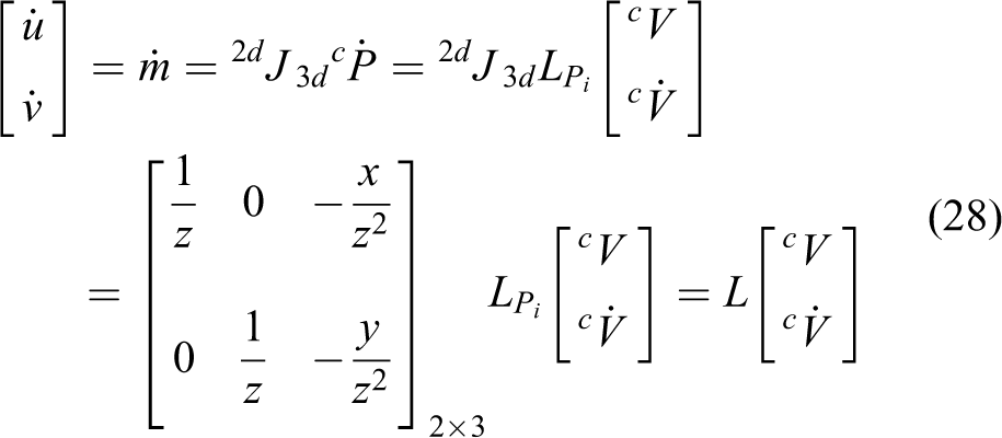
The derivation of the image Jacobian matrix is elaborated in the following. A three-dimensional (3D) feature point ${}^{c}P = {[{}^{c}x, {}^{c}y, {}^{c}z]}^{T}$ in the camera frame and its corresponding image feature point $f = {[u, v]}^{T}$ on the image plane is given. In addition, we also assume that the camera has zero skew, that is, δ = 0. As a result, equation (1) can be rewritten as

f = [\begin{array}{l} u \\ v \end{array}] = [\begin{array}{l} \frac{λ_{x} {}^{c}x}{{}^{c}z} + u_{0} \\ \frac{λ_{y} {}^{c}y}{{}^{c}z} + v_{0} \end{array}]

Differentiating equation (6) with respect to time will yield

\dot{f} = [\begin{array}{l} \dot{u} \\ \dot{v} \end{array}] = [\begin{array}{l} λ_{x} \frac{{}^{c}z {}^{c}{\dot{x}} - {}^{c}x {}^{c}{\dot{z}}}{z^{2}} \\ λ_{y} \frac{{}^{c}z {}^{c}{\dot{y}} - {}^{c}y {}^{c}{\dot{z}}}{{{}^{c}z}^{2}} \end{array}]

Suppose that this 3D point undergoes a rigid body motion. One will have

{}^{c}{\dot{P}} = {}^{c}υ + {}^{c}ω \times {}^{c}P

where ${}^{c}υ = {[\begin{matrix} {{}^{c}υ}_{x} & {{}^{c}υ}_{y} & {{}^{c}υ}_{z} \end{matrix}]}^{T}$ and ${}^{c}ω = {[\begin{matrix} {{}^{c}ω}_{x} & {{}^{c}ω}_{y} & {{}^{c}ω}_{z} \end{matrix}]}^{T}$ .

Developing equation (8) will yield

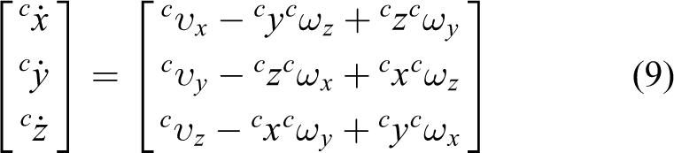
[\begin{matrix} {}^{c}{\dot{x}} \\ {}^{c}{\dot{y}} \\ {}^{c}{\dot{z}} \end{matrix}] = [\begin{matrix} {{}^{c}υ}_{x} - {}^{c}y {{}^{c}ω}_{z} + {}^{c}z {{}^{c}ω}_{y} \\ {{}^{c}υ}_{y} - {}^{c}z {{}^{c}ω}_{x} + {}^{c}x {{}^{c}ω}_{z} \\ {{}^{c}υ}_{z} - {}^{c}x {{}^{c}ω}_{y} + {}^{c}y {{}^{c}ω}_{x} \end{matrix}]

Substituting equation (9) into equation (7) and rearranging terms will result in

\dot{f} = [\begin{matrix} \dot{u} \\ \dot{v} \end{matrix}] = [\begin{matrix} \frac{λ_{x}}{{}^{c}z} & 0 & - \frac{(u - u_{0})}{{}^{c}z} & - \frac{(u - u_{0}) (v - v_{0})}{λ_{y}} & \frac{{λ_{x}}^{2} + {(u - u_{0})}^{2}}{λ_{x}} & - λ_{x} \frac{(v - v_{0})}{λ_{y}} \\ 0 & \frac{λ_{y}}{{}^{c}z} & - \frac{(v - v_{0})}{{}^{c}z} & - \frac{{λ_{y}}^{2} + {(v - v_{0})}^{2}}{λ_{y}} & \frac{(u - u_{0}) (v - v_{0})}{λ_{x}} & λ_{y} \frac{(u - u_{0})}{λ_{x}} \end{matrix}] [\begin{matrix} {{}^{c}υ}_{x} \\ {{}^{c}υ}_{y} \\ {{}^{c}υ}_{z} \\ {{}^{c}ω}_{x} \\ {{}^{c}ω}_{y} \\ {{}^{c}ω}_{z} \end{matrix}]

Equation ( 10) can be further expressed as

\dot{f} = L_{e} {}^{c}V = L_{e} [\begin{matrix} {}^{c}υ \\ {}^{c}ω \end{matrix}]

Depth and velocity estimation based on Kalman filter and virtual visual servoing

The image Jacobian matrix described by equation (10) consists of five parameters— $λ_{x}$ , $λ_{y}$ , u, v, and ${}^{c}z$ . However, in practice, the depth value ${}^{c}z$ of an object point (i.e. feature point) is not often available. Common approaches to coping with this problem including the design of a depth observer or the use of stereo cameras. In this article, a novel approach based on the concept of virtual visual servoing¹⁸ and Kalman filter²¹ is developed to estimate the depth value that is essential in calculating the image Jacobian matrix.

The idea of virtual visual servoing proposed by Marchan and Chaumette¹⁸ was originally used in augmented reality applications. Since the virtual image must appear at the correct position in the real scene in augmented reality applications, the relationship between the camera frame and the real object is therefore crucial. That is, the calibration accuracy of extrinsic camera parameters is very important. The concept of virtual visual servoing¹³ is illustrated in Figure 2 and will be elaborated in the next subsection.

Figure 2.

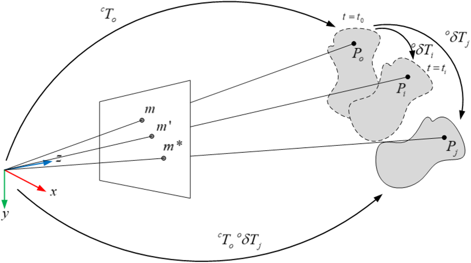
Concept of virtual visual servoing.

Pose and velocity estimation based on virtual visual servoing

In Figure 2, $m^{*} = {[u^{*}, v^{*}]}^{T}$ represents the image point on the image plane corresponding to the actual object point P_j , and $m = {[u, v]}^{T}$ represents the image point on the image plane corresponding to the virtual object point P_o before updating the extrinsic camera parameters. If the motion of the camera is properly controlled so that P_o converges to P_j , one can expect that m will converge to m* as well; namely, ${}^{o}δ T_{j}$ can be found. Since the position of the point P_o is randomly initialized, ${{}^{c}T}_{o}$ is therefore known. As a result, one can obtain accurate extrinsic camera parameters ${{}^{c}T}_{o} {}^{o}δ T_{j}$ as well as ${}^{o}δ T_{j}$ . The concept of IBVS is exploited to find ${}^{o}δ T_{j}$ . Similar to the derivation of equations (10) and (11), one can calculate the corresponding image Jacobian L that describes the relationship between the virtual velocity screw ${{}^{c}V}_{vir} = {[\begin{matrix} υ^{T} (t) & ω^{T} (t) \end{matrix}]}^{T}$ of P_o and the time derivative of image feature m using the following equation

\dot{m} = L {{}^{c}V}_{vir}

The image feature error e _vir between m and m* is defined as

e_{vir} = m - m^{*}

If the goal is to exponentially converge e _vir, one can let

{\dot{e}}_{vir} = - K e_{vir}, K > 0

Substituting equation (13) into equation (14) will yield

\dot{m} - {\dot{m}}^{*} = - K (m - m^{*})

Substituting equation (12) into equation (15) will yield

L {{}^{c}V}_{v i r} - {\dot{m}}^{*} = - K (m - m^{*})

From equation (16), one will have

{{}^{c}V}_{v i r} = - K L^{+} (m - m^{*}) + L^{+} {\dot{m}}^{*}

As shown in Figure 2, the rigid transformation ${}^{o}δ T_{i}$ consists of the translation increment $δ P_{i}$ and the rotation increment $δ θ_{i}$ described by equations (18) and (19), respectively. Note that t_i − t ₀ = i▵t, where ▵t in equations (18) and (19) is the sampling time

δ P_{i} = \int_{t_{o}}^{t_{i}} υ (t) d t \approx \sum_{k = 0}^{i - 1} υ_{k} Δ t

δ θ_{i} = \int_{t_{o}}^{t_{i}} ω (t) d t \approx \sum_{k = 0}^{i - 1} ω_{k} Δ t

Note that $δ θ_{i}$ is the rotation increment around a specific axis and its corresponding rotation matrix $δ R_{i}$ can be obtained using the Rodrigues formula²⁸ or alternatively using the exponential matrix map described by the following equation

δ R_{i} = exp ({[δ θ_{i}]}_{\times})

As illustrated in Figure 2, after the time duration t_i − t ₀ had passed, the original image point m moved to the new image point $m'$ . The original virtual object point P_o is updated to P_i by repeating using equations (12) –(20). Eventually, the image point will converge to $m^{*}$ , while the virtual object point will converge to P_j .

One interesting application of virtual visual servoing is that it can be used to estimate the velocity of the actual object point P_j . The idea is to integrate the virtual velocity screw ${{}^{c}V}_{vir}$ within a fixed time interval ▵t. By properly adjusting the value of gain constant K in equation (17), it is possible to obtain a specific ${{}^{c}V}_{vir}$ so that the resulting rigid transformation will be very close to ${}^{o}δ T_{j}$ . That is, m will converge to m* and P_o will converge to P_j within one sampling time period. In this case, the virtual velocity screw at P_o will be very close to the velocity screw at P_j .

To improve the depth estimation accuracy, the acceleration information of the virtual object point P_o in the camera frame can be taken into consideration.¹³ Detailed derivations are provided in the following.

Suppose that the virtual object point P_o undergoes a rigid body motion,²⁹ one will have

{}^{c}{\dot{P}} (t_{0}) = {}^{c}υ + {}^{c}ω \times {}^{c}P

To obtain the acceleration term, one can differentiate equation (21) with respect to time to get

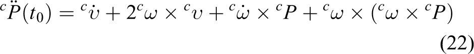
{}^{c}{\ddot{P}} (t_{0}) = {}^{c}{\dot{υ}} + 2 {}^{c}ω \times {}^{c}υ + {}^{c}{\dot{ω}} \times {}^{c}P + {}^{c}ω \times ({}^{c}ω \times {}^{c}P)

Suppose that the sampling time ▵t is very small. The velocity information of the virtual object point P_o in the camera frame at time instant t ₀ + ▵t can be approximated as

{}^{c}{\dot{P}} (t_{0} + Δ t) \approx {}^{c}{\dot{P}} (t_{0}) + Δ t {}^{c}{\ddot{P}} (t_{0})

Substituting equations (21) and (22) into equation (23) will yield

{}^{c}{\dot{P}} (t_{0}) + Δ t {}^{c}{\ddot{P}} (t_{0}) = {}^{c}υ + {}^{c}ω \times {}^{c}P + Δ t ({}^{c}{\dot{υ}} + 2 {}^{c}ω \times {}^{c}υ + {}^{c}{\dot{ω}} \times {}^{c}P + {}^{c}ω \times ({}^{c}ω \times {}^{c}P))

Equation ( 24) can be rewritten as

\begin{array}{l} {}^{c}{\dot{P}} (t_{0}) + Δ t {}^{c}{\ddot{P}} (t_{0}) \\ = {}^{c}υ + {[{}^{c}ω]}_{\times} {}^{c}P + Δ t ({}^{c}{\dot{υ}} + 2 {[{}^{c}ω]}_{\times} {}^{c}υ + {[{}^{c}{\dot{ω}}]}_{\times} {}^{c}P + {[{}^{c}ω]}_{\times} ({[{}^{c}ω]}_{\times} {}^{c}P)) \end{array}

After some manipulations, equation (25) can be further expressed as

\begin{array}{l} {}^{c}{\dot{P}} (t_{0}) + Δ t {}^{c}{\ddot{P}} (t_{0}) \\ = {}^{c}υ + 2 Δ t {[{}^{c}ω]}_{\times} {}^{c}υ + Δ t {}^{c}{\dot{υ}} - {[{}^{c}P]}_{\times} {}^{c}ω + Δ t {[{[{}^{c}P]}_{\times} {}^{c}ω]}_{\times} {}^{c}ω - Δ t {[{}^{c}P]}_{\times} {}^{c}{\dot{ω}} \end{array}

Equation (26) can be expressed in matrix form as

\begin{array}{l} {}^{c}{\dot{P}} (t_{0} + Δ t) \approx {}^{c}{\dot{P}} (t_{0}) + Δ t {}^{c}{\ddot{P}} (t_{0}) \\ = {[I + 2 Δ t {[{}^{c}ω]}_{\times} - {[{}^{c}P]}_{\times} + Δ t {[{[{}^{c}P]}_{\times} {}^{c}ω]}_{\times} Δ t \cdot I - Δ t {[{}^{c}P]}_{\times}]}_{3 \times 12} {[\begin{array}{l} {}^{c}υ \\ {}^{c}ω \\ {}^{c}{\dot{υ}} \\ {}^{c}{\dot{ω}} \end{array}]}_{12 \times 1} \\ = L_{P_{i}} [\begin{array}{l} {}^{c}V \\ {}^{c}{\dot{V}} \end{array}] \end{array}

Equation ( 27) describes the relationship between the velocity ${}^{c}{\dot{P}}$ in the camera frame and ${[\begin{matrix} {{}^{c}V}^{T} & {}^{c}{\dot{V}}^{T} \end{matrix}]}^{T}$ . In addition, the relationship between $\dot{m}$ and ${[\begin{matrix} {{}^{c}V}^{T} & {}^{c}{\dot{V}}^{T} \end{matrix}]}^{T}$ is described by the following equation

[\begin{array}{l} \dot{u} \\ \dot{v} \end{array}] = \dot{m} = {{}^{2 d}J}_{3 d} {}^{c}{\dot{P}} = {{}^{2 d}J}_{3 d} L_{P_{i}} [\begin{array}{l} {}^{c}V \\ {}^{c}{\dot{V}} \end{array}] = {[\begin{matrix} \frac{1}{z} & 0 & - \frac{x}{z^{2}} \\ 0 & \frac{1}{z} & - \frac{y}{z^{2}} \end{matrix}]}_{2 \times 3} L_{P_{i}} [\begin{array}{l} {}^{c}V \\ {}^{c}{\dot{V}} \end{array}] = L [\begin{array}{l} {}^{c}V \\ {}^{c}{\dot{V}} \end{array}]

With the consideration of the acceleration term, equations (18) and (19) can be rewritten as

δ P_{i} = \int_{t_{o}}^{t_{i}} υ (t) d t = \sum_{k = 0}^{i - 1} (υ_{k} Δ t + \frac{1}{2} {\dot{υ}}_{k} {(Δ t)}^{2})

δ θ_{i} = \sum_{k = 0}^{i - 1} (ω_{k} Δ t + \frac{1}{2} {\dot{ω}}_{k} {(Δ t)}^{2})

Depth and velocity estimation based on Kalman filter and virtual visual servoing

Considering the fact that the captured image often contains noise and there are limitations on computational resources and camera sampling rate, this article proposes a depth and velocity estimator that combines the Kalman filter with the virtual visual servoing technique so as to reduce noise effects and also improve estimation accuracy. Figure 3 shows the schematic diagram of the proposed depth and velocity estimator.

Figure 3.

Schematic diagram of the proposed depth and velocity estimator based on Kalman filter and virtual visual servoing.

The discrete-time state equation and output equation of a typical dynamic system can be expressed as

X (k + 1) = A_{d} X (k) + B_{d} U (k) + ξ (k)

Y (k) = C_{d} X (k) + η (k)

where X(k) is the state vector, U(k) is the input vector, and Y(k) is the output vector; ξ(k) is the process noise vector and η(k) is the measurement noise vector; and A_d , B_d , and C_d are constant matrices of proper dimensions. In this article, the process noise vector ξ(k) is assumed to be a zero vector.

The position and velocity of the actual object point P_j in the camera frame are defined as the state variables X(k) in equation (33). In addition, the acceleration of the actual object point P_j in the camera frame is defined as the input U(k) (equation (33)) to the system

X (k) = [\begin{array}{l} x (k) \\ y (k) \\ z (k) \\ v_{x} (k) \\ v_{y} (k) \\ v_{z} (k) \end{array}], U (k) = [\begin{array}{l} U_{x} (k) \\ U_{y} (k) \\ U_{z} (k) \end{array}]

A_d and B_d in equation (31) are described by the following equation

A_{d} = [\begin{matrix} 1 & 0 & 0 & Δ t & 0 & 0 \\ 0 & 1 & 0 & 0 & Δ t & 0 \\ 0 & 0 & 1 & 0 & 0 & Δ t \\ 0 & 0 & 0 & 1 & 0 & 0 \\ 0 & 0 & 0 & 0 & 1 & 0 \\ 0 & 0 & 0 & 0 & 0 & 1 \end{matrix}], B_{d} = [\begin{matrix} 0.5 {(Δ t)}^{2} & 0 & 0 \\ 0 & 0.5 {(Δ t)}^{2} & 0 \\ 0 & 0 & 0.5 {(Δ t)}^{2} \\ Δ t & 0 & 0 \\ 0 & Δ t & 0 \\ 0 & 0 & Δ t \end{matrix}]

That is

[\begin{array}{l} x (k +1) \\ y (k +1) \\ z (k +1) \\ υ_{x} (k +1) \\ υ_{y} (k +1) \\ υ_{z} (k +1) \end{array}] = [\begin{matrix} 1 & 0 & 0 & Δ t & 0 & 0 \\ 0 & 1 & 0 & 0 & Δ t & 0 \\ 0 & 0 & 1 & 0 & 0 & Δ t \\ 0 & 0 & 0 & 1 & 0 & 0 \\ 0 & 0 & 0 & 0 & 1 & 0 \\ 0 & 0 & 0 & 0 & 0 & 1 \end{matrix}] [\begin{array}{l} x (k) \\ y (k) \\ z (k) \\ υ_{x} (k) \\ υ_{y} (k) \\ υ_{z} (k) \end{array}] + [\begin{matrix} 0.5 {(Δ t)}^{2} & 0 & 0 \\ 0 & 0.5 {(Δ t)}^{2} & 0 \\ 0 & 0 & 0.5 {(Δ t)}^{2} \\ Δ t & 0 & 0 \\ 0 & Δ t & 0 \\ 0 & 0 & Δ t \end{matrix}] [\begin{array}{l} U_{x} (k) \\ U_{y} (k) \\ U_{z} (k) \end{array}]

In the following, we will determine the transformation matrix C_d between the system states $\hat{X} (k)$ and the measured output Y(k). The system states x(k), y(k), and z(k) can be estimated by using perspective projection, current image point $m^{*}$ , previous estimated depth value z(k−1), and the virtual servoing technique. In addition, the other three system states $υ_{x} (k)$ , $υ_{y} (k)$ , and $υ_{z} (k)$ can be estimated using the virtual servoing technique. Since all the states can be either directly or indirectly estimated/measured, C_d is an identity matrix. Therefore

Y (k) = C_{d} X (k) + η (k) = [\begin{matrix} 1 & 0 & 0 & 0 & 0 & 0 \\ 0 & 1 & 0 & 0 & 0 & 0 \\ 0 & 0 & 1 & 0 & 0 & 0 \\ 0 & 0 & 0 & 1 & 0 & 0 \\ 0 & 0 & 0 & 0 & 1 & 0 \\ 0 & 0 & 0 & 0 & 0 & 1 \end{matrix}] [\begin{array}{l} x (k) \\ y (k) \\ z (k) \\ υ_{x} (k) \\ υ_{y} (k) \\ υ_{z} (k) \end{array}] + η (k)

The Kalman filter-based depth and velocity estimator is implemented using equations (33) –(37)

\{\begin{matrix} {\hat{X}}^{-} (k + 1) = A_{d} \hat{X} (k) + B_{d} U (k) \\ Σ^{-} (k +1) = A_{d} Σ (k) A_{d}^{T} + Q \\ K (k +1) = Σ^{-} (k + 1) C_{d}^{T} {(C_{d} Σ^{-} (k + 1) C_{d}^{T} + R)}^{- 1} \\ \hat{X} (k +1) = {\hat{X}}^{-} (k +1) + K (k + 1) (Y (k + 1) - C_{d} {\hat{X}}^{-} (k +1)) \\ Σ (k +1) = (I - K (k + 1) C_{d}) Σ^{-} (k +1) \end{matrix}

where K(k) is the Kalman filter gain matrix and Σ(k) is the covariance matrix for the state estimate $\hat{X} (k)$ . Equation (37) gives the state estimate; namely, the depth value and velocity can be estimated.

In this article, the covariance matrix R for the measurement noise η(k) is determined through a trial-and-error manner, whereas the covariance matrix Q for the process noise ξ(k) is set to a null matrix in equation (37). The proposed depth and velocity estimator that combines the Kalman filter with the virtual visual servoing technique is easy to implement. It is used in the proposed MIBDVS architecture that will be investigated in the next section. In particular, the proposed Kalman filter-based depth and velocity estimator is used in the MIBDVS architecture to estimate the parameter values of the interaction matrix. It is worth noting that the virtual visual servoing technique exploits the idea of IBVS. As a result, the virtual visual servoing technique inherits the drawbacks of IBVS as well. For instance, if the straight line that passes the real object point and the virtual object point is parallel with the optical axis, then their corresponding image points on the image plane will coincide with each other. In this case, it is impossible to exploit the error between these two image points to estimate the position/velocity of the real object point. Nevertheless, the user can choose the initial position of the virtual object point to avoid such a case happening.

Dynamic visual servoing

Dynamic model of a 2-DOF planar robot manipulator and CTC

The dynamic model of a 2-DOF planar robot manipulator can be described by

M (q) \ddot{q} + C (q, \dot{q}) \dot{q} + F (\dot{q}) = τ

where τ is the 2 × 1 torque vector; M(q) and $C (q, \dot{q})$ are the 2 × 2 inertia matrix and Coriolis matrix, respectively; $F (\dot{q})$ is the 2 × 1 friction vector; and q is the 2 × 1 generalized coordinate (in this article, q is the 2 × 1 joint angle vector).

Unlike most classical visual servoing schemes which only use a proportional-type feedback control law, both IBDVS and the proposed MIBDVS exploit the idea of CTC.^15,30,31 In general, the CTC law τ _ctc can be expressed as

τ_{ctc} = \hat{M} (q) [{\ddot{q}}_{d} + K_{D} \dot{e} + K_{P} e] + \hat{C} (q, \dot{q}) \dot{q} + \hat{F} (\dot{q})

where $\hat{M} (q)$ , $\hat{C} (q, \dot{q})$ , and $\hat{F} (\dot{q})$ are the estimated inertia matrix, Coriolis matrix, and friction vector, respectively, as obtained through system identification^32,33; q_d is the 2 × 1 desired joint angle vector; e_q = q − q_d is the 2 × 1 joint angle error vector; K_D is the 2 × 2 constant derivative gain diagonal matrix; and K_P is the 2 × 2 constant proportional gain diagonal matrix.

Suppose that the system identification results are perfect; that is, $\hat{M} (q) = M (q)$ , $\hat{C} (q, \dot{q}) = C (q, \dot{q})$ , $\hat{F} (\dot{q}) = F (\dot{q})$ .

Letting τ in equation (38) be equal to τ _ctc described by equation (39) will yield

M (q) [{\ddot{q}}_{d} - \ddot{q} + K_{D} {\dot{e}}_{q} + K_{P} e_{q}] = 0

Since the inertia matrix M(q) is a nonsingular square matrix, multiplying the inverse matrix of M(q) on both sides of equation (40) will lead to

{\ddot{e}}_{q} + K_{D} {\dot{e}}_{q} + K_{P} e_{q} = 0

One interesting observation is that the CTC method can yield satisfactory performance if the dynamic model obtained through system identification is accurate. However, if the identified dynamic model is not accurate, then the CTC method may result in poor control performance. Figure 4 shows a typical block diagram of CTC.

Figure 4.

Typical block diagram of CTC. CTC: computed torque control.

IBDVS and the proposed MIBDVS

Figure 5 illustrates the control block diagram of IBDVS. The IBDVS incorporates a depth and velocity estimator, a second-order visual loop controller, and a robot control loop that uses the position feedback provided by the encoder. The IBDVS architecture is similar to the classical IBVS architecture. Both the IBDVS architecture and the classical IBVS architecture use the image feature command for the visual loop. The difference is that in the IBDVS architecture, the velocity loop of the robot control architecture adopts the CTC scheme rather than the conventional feedback controller. However, as shown in Figure 5, the IBDVS architecture only provides the desired joint acceleration command ${\ddot{q}}_{d}$ for the CTC scheme from the visual loop. That is, the desired joint angle command q_d and the desired joint velocity command ${\dot{q}}_{d}$ are completely ignored. It is not a common way to implement CTC. Therefore, to cope with this problem, in this article,q_d , ${\dot{q}}_{d}$ , and ${\ddot{q}}_{d}$ are all used in the CTC scheme. The modified visual servoing architecture is called MIBDVS in this article. Figure 6 shows the block diagram of the proposed MIBDVS architecture. Note that in the proposed MIBDVS architecture, the depth and velocity estimator is implemented based on the Kalman filter.

Figure 5.

Control block diagram of IBDVS. IBDVS: image-based dynamic visual servoing.

Figure 6.

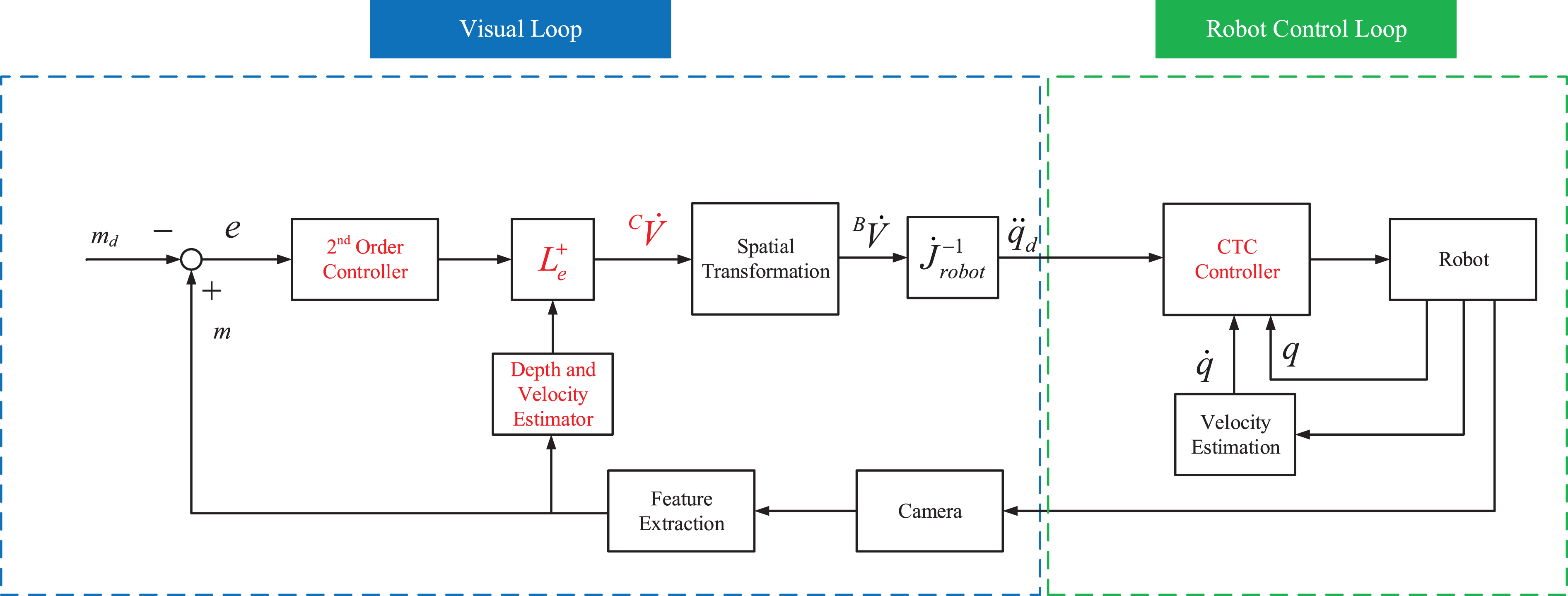
Control block diagram of the proposed MIBDVS. MIBDVS: modified image-based dynamic visual servoing.

In Figure 6, the depth and velocity estimator estimates the parameter values essential in the calculation of interaction matrix $\hat{L}$ , and $IDM (\hat{q}, \hat{\dot{q}})$ is the inverse dynamic model.¹³ Figure 7 shows the detailed computations of the commands used in the proposed MIBDVS architecture. As shown in Figure 7, using the Kalman filter-based depth and velocity estimator and the image feature $\hat{m}$ , the position feedback needed in the CTC scheme can be obtained.

Figure 7.

Derivation of position command used in the CTC scheme.CTC: computed torque control.

Controller design of MIBDVS

The controller design of the MIBDVS architecture in Figure 6 will be explicated in the following. The task function E is defined by equation (42), where $e = m - m_{d} = {[u - u_{d}, v - v_{d}]}^{T}$ represents the image feature error

E = \int e d t

Suppose that the goal is to converge image feature error to behave as a second-order system. As a result, one will have equation (43), where $Λ_{v}$ and $Λ_{p}$ are suitable gains designed by users

\ddot{E} + Λ_{v} \dot{E} + Λ_{p} E = 0

Substituting equation (42) into equation (43) will yield

\begin{array}{l} \dot{e} + Λ_{v} e + Λ_{p} \int e d t = 0 \\ \Rightarrow (\dot{m} - {\dot{m}}_{d}) + Λ_{v} (m - m_{d}) + Λ_{p} \int (m - m_{d}) d t = 0 \end{array}

The velocity command ${}^{c}V$ and acceleration command ${}^{c}{\dot{V}}$ are obtained by equations (28) and (44) as follows

\begin{array}{l} L [\begin{array}{l} {}^{c}V \\ {}^{c}{\dot{V}} \end{array}] - {\dot{m}}_{d} + Λ_{v} (m - m_{d}) + Λ_{p} \int (m - m_{d}) d t = 0 \\ \Rightarrow [\begin{array}{l} {}^{c}V \\ {}^{c}{\dot{V}} \end{array}] = L^{+} [{\dot{m}}_{d} - Λ_{v} (m - m_{d}) - Λ_{p} \int (m - m_{d}) d t] \end{array}

Image feature command generation and interpolation

In the experiment, the image feature command is generated through the so-called teach by showing method. During the “teach by showing” stage, the user holds and moves a fiducial marker to the goal position and the camera is used to record the entire moving trajectory of the fiducial marker. In the “execution” stage, the recorded moving trajectory is adopted as the image feature command for the visual servoing scheme and the selective compliance assembly robot arm (SCARA) robot is controlled to repeat (i.e. move along) the recorded moving trajectory. Note that in this article, the recorded moving trajectory is represented by a PH curve.^34,35

Experimental setup and results

Figure 8 shows the experimental system that consists of a 2-DOF SCARA robot (as shown in Figure 9), two eye-to-hand cameras (mounted on the ceiling as shown in Figure 10), a personal computer, and an intelligent motion control platform-2 card by Industrial Technology Research Institute, Zhudong Township. Note that two eye-to-hand cameras are used in the hand–eye calibration process³⁶ (for later use in the joint velocity estimation experiment). When performing visual servoing, only the left eye-to-hand camera (the camera denoted as “L” in Figure 10) is used. The two joints of the planar robot are actuated by two AC servomotors and the motor drives are set to torque mode throughout the experiments. In particular, the “L” eye-to-hand camera, which is equipped with a lens of 16 mm focus length, has a maximum resolution of 1280 × 1024 pixel² and 60 Hz frame rate. In addition, the distance (measured by a ruler) between the “L” eye-to-hand camera and the 2-DOF SCARA robot is around 135 cm.

Figure 8.

Experimental system.

Figure 9.

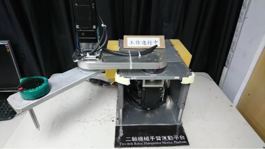
2-DOF SCARA robot. DOF: degree of freedom; SCARA: selective compliance assembly robot arm.

Figure 10.

Eye-to-hand camera mounted on the ceiling.

Experimental results of Kalman filter-based joint velocity estimation

In this experiment, the SCARA robot is controlled to perform a contour following motion. Three different approaches—the depth and velocity estimator without incorporating the Kalman filter, the proposed Kalman filter-based depth and velocity estimator, and the least square fit (LSF) method³⁷—are used to estimate the joint velocity of the robot. In particular, the LSF method uses the encoder data of the servomotor installed at each joint to estimate the joint velocity, whereas the other two approaches only use the image information obtained by the camera to estimate the joint velocity. Since the resolution of the encoder data is much higher than that of the image data provided by the camera, it is expected that the estimation accuracy of the LSF method will be better than the other two approaches. Therefore, the estimation results of the LSF method will be used as a reference to assess the estimation accuracy of the proposed Kalman filter-based depth and velocity estimator in addition to the depth and velocity estimator without incorporating the Kalman filter. Note that in this experiment, the object feature point is on the tip of the second joint (i.e. end-effector). The depth and velocity estimator without incorporating the Kalman filter as well as the proposed Kalman filter-based depth and velocity estimator can estimate the velocity of the end-effector in the camera frame using image information only. By exploiting the results of hand–eye calibration and inverse robot Jacobian, one can convert the velocity of the end-effector in the camera frame into the joint velocity of the robot.

According to the joint velocity estimation results shown in Figures 11 and 12, the estimation performance of the proposed Kalman filter-based depth and velocity estimator is clearly better than that of the depth and velocity estimator without incorporating the Kalman filter.

Figure 11.

Velocity estimation result of the first joint. (a) depth and velocity estimator without incorporating the Kalman filter and (b) proposed Kalman filter-based depth and velocity estimator.

Figure 12.

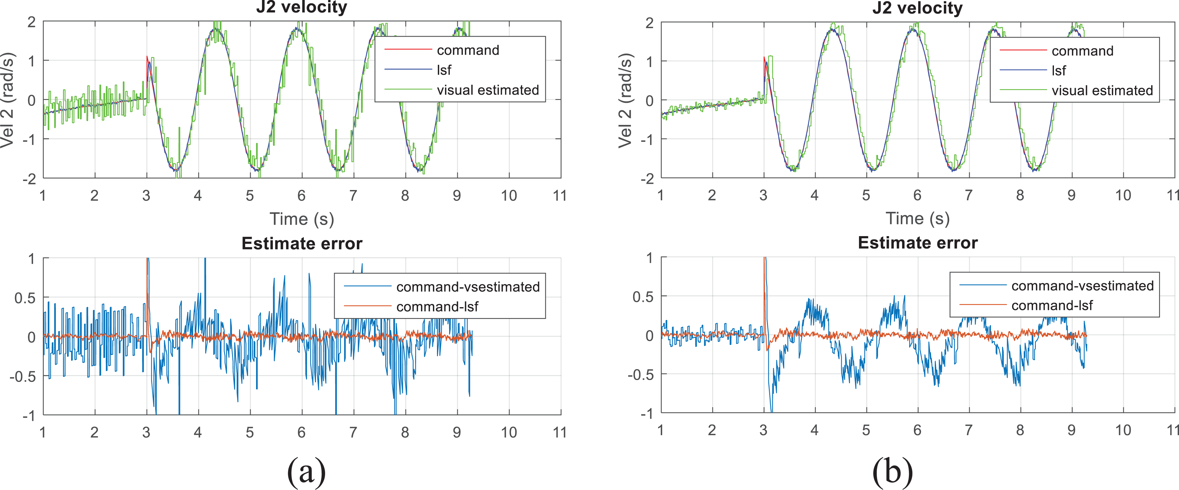
Velocity estimation result of the second joint: (a) depth and velocity estimator without incorporating the Kalman filter and (b) proposed Kalman filter-based depth and velocity estimator.

Experimental results of Kalman filter-based depth estimation

In this experiment, the SCARA robot is controlled to perform a contour following motion. Two different approaches—the proposed Kalman filter-based depth and velocity estimator and the depth and velocity estimator without incorporating the Kalman filter—are tested in the experiment. Note that in this experiment, the depth of the robot is estimated using the image information only. In addition, the ground truth of the object depth measured by a ruler is around 135 cm. Results of the depth estimation experiment are shown in Figure 13. Clearly, the proposed Kalman filter-based depth and velocity estimator exhibits better depth estimation accuracy than the depth and velocity estimator without incorporating the Kalman filter.

Figure 13.

Depth estimation result: (a) depth and velocity estimator without incorporating the Kalman filter and (b) proposed Kalman filter-based depth and velocity estimator.

Comparison of tracking performance between IBVS and MIBDVS

In this experiment, the SCARA robot is controlled to perform a contour following motion. Both the classical IBVS and the proposed MIBDVS are tested. Figure 14 shows the desired contour. Figure 15 shows the image command after interpolation, whereas Figure 16 shows the image velocity command. Tracking results on the image plane are shown in Figure 17, whereas Figure 18 shows the tracking errors of the image features. In addition, the performance comparison between the classical IBVS and the proposed MIBDVS is summarized in Table 1, where “RMS” represents the root-mean-square value and “MAX” is the maximum value. Based on Table 1, clearly, both the RMS values and the MAX values of tracking error on the u-axis and v-axis for the case of the proposed MIBDVS are smaller than those for the case of the classical IBVS. In addition to tracking error, contour error—an important indicator of contour following accuracy—is also compared. Again, both the RMS values and the MAX values of contour error for the case of the proposed MIBDVS are smaller than those for the case of the classical IBVS. Experimental results indicate that the proposed MIBDVS structure outperforms the classical IBVS structure in both tracking performance and contour following accuracy.

Figure 14.

Desired contour; red line: the recorded moving trajectory of the fiducial marker during the “teach by showing” stage and blue line: the desired contour, which is a PH curve used to represent (i.e. fit) the recorded moving trajectory.

Figure 15.

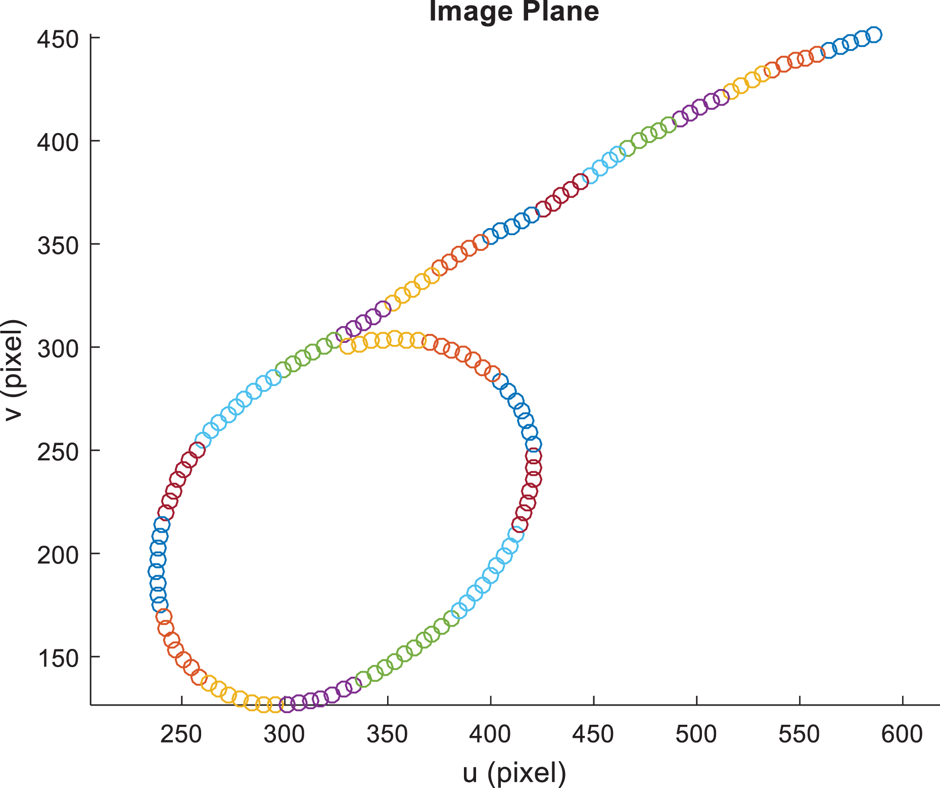
Image command after interpolation.

Figure 16.

Image velocity command.

Figure 17.

Tracking results on the image plane: (a) IBVS and (b) MIBDVS. IBVS: image-based visual servoing; MIBDVS: modified image-based dynamic visual servoing.

Figure 18.

Tracking error of image feature: (a) IBVS and (b) MIBDVS. IBVS: image-based visual servoing; MIBDVS: modified image-based dynamic visual servoing.

Table 1.

Performance comparison between IBVS and MIBDVS.

	u-axis tracking error (pixel)		v-axis tracking error (pixel)		contour error (pixel)
	RMS	MAX	RMS	MAX	RMS	MAX
IBVS	3.6546	9.6489	3.2264	8.3667	2.3514	5.9492
MIBDVS	1.8224	8.1785	1.3193	4.2363	1.9770	4.9546

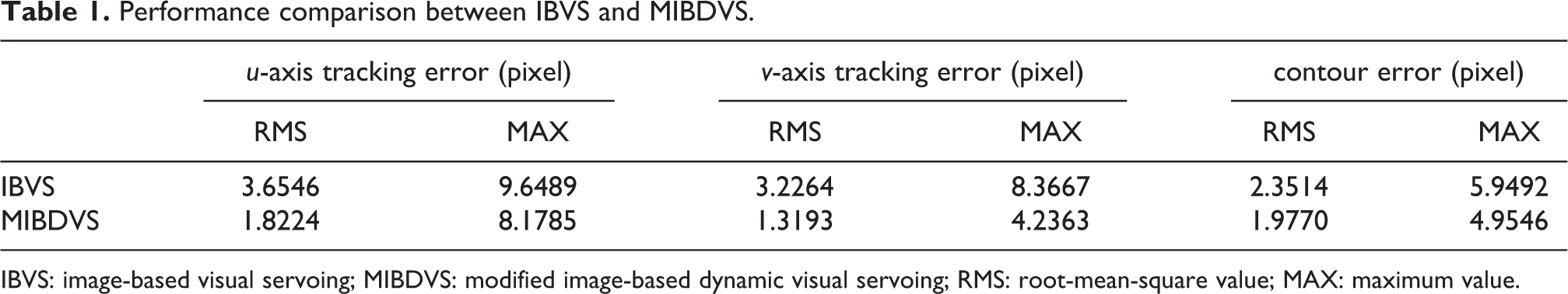
IBVS: image-based visual servoing; MIBDVS: modified image-based dynamic visual servoing; RMS: root-mean-square value; MAX: maximum value.

Conclusions

This article exploits the concept of virtual visual servoing and Kalman filter to develop a method for estimating the depth value that is essential in calculating the image Jacobian matrix used in IBVS architectures. In particular, the Kalman filter is employed to cope with image noise so as to improve the accuracy of depth estimation. In addition, the proposed Kalman filter-based approach is also employed to estimate the joint velocity of the robot using image information only. Moreover, to achieve better visual servoing performance, this article proposes the MIBDVS architecture that exploits the desired joint angle command, the desired joint velocity command, and the desired joint acceleration command in the implementation of the CTC scheme. Several experiments conducted on a 2-DOF planar manipulator are used to evaluate the performance of the proposed Kalman filter-based depth and velocity estimator and the proposed MIBDVS architecture. Experimental results indicate that the two proposed approaches outperform the ones based on the classical IBVS architecture.

In this article, the inertia matrix, Coriolis matrix, and friction vector, which are essential in the implementation of the CTC scheme, are obtained through system identification. However, the accuracy of the identification results of these matrices/vectors greatly affects the effectiveness of the CTC scheme as well as that of the proposed MIBDVS architecture. Improving identification accuracy is one possible future direction. In addition, the sampling rate for the inner servo control loop is often more than 10 times that for the outer vision loop. This results in a major challenge for the control design of MIBDVS. How to ease this difficulty so as to facilitate the control design of MIBDVS is another possible research direction.

Footnotes

Declaration of conflicting interests

The author(s) declared no potential conflicts of interest with respect to the research, authorship, and/or publication of this article.

Funding

The author(s) disclosed receipt of the following financial support for the research, authorship, and/or publication of this article: The project is supported by the Ministry of Science and Technology, Taiwan, under MOST 105-2221-E-006-105-MY3.

ORCID iD

Ming-Yang Cheng

References

Hill

Park

. Real time control of a robot with a mobile camera. In: Proceedings of 9th ISIR, Washington, USA, March 1979, pp. 233–246.

Weiss

Sanderson

Neuman

. Dynamic sensor-based control of robots with visual feedback. IEEE J Robot Autom 1987; 3(5): 404–417.

Hutchinson

Hager

Corke

. A tutorial on visual servo control. IEEE Trans Robot Autom 1996; 12(5): 651–670.

Chaumette

Hutchinson

. Visual servo control part I: basic approaches. IEEE Robot Autom Mag 2006; 13(4): 82–90.

Chaumette

Hutchinson

. Visual servo control, part II: advanced approaches. IEEE Robot Autom Mag 2007; 14(1): 109–118.

Corke

PI.

Dynamic issues in robot visual-servo systems. In: Proceedings of symposium robotics research, Herrsching, Germany, 1995, pp. 488–498.

Corke

Good

. Dynamic effects in visual closed-loop systems. IEEE Trans Robot Autom 1996; 12(5): 671–683.

Wang

Lang

Silva

CWD

. A hybrid visual servo controller for robust grasping by wheeled mobile robots. IEEE/ASME Trans Mech 2010; 15(5): 757–769.

Siradjuddin

Behera

McGinnity

, et al. Image-based visual servoing of a 7-DOF robot manipulator using an adaptive distributed fuzzy PD controller. IEEE/ASME Trans Mech 2014; 19(2): 512–523.

10.

Shi

Hwang

, et al. Decoupled visual servoing with fuzzy Q-learning. IEEE Trans Ind Inform 2018; 14(1): 241–252.

11.

Belmonte

Ramón

Pomares

, et al. Optimal image-based guidance of mobile manipulators using direct visual servoing. Electronics 2019; 8(4): 374.

12.

Xin

Cheng

Ran

. Visual servoing of robot manipulator with weak field-of-view constraints. Int J Adv Robot Syst 2021; 18(1): 1–11.

13.

Dahmouche

Andreff

Mezouar

. Dynamic visual servoing from sequential regions of interest acquisition. Int J Robot Res 2012; 31(4): 520–537.

14.

Keshmiri

Xie

Mohebbi

. Augmented image-based visual servoing of a manipulator using acceleration command. IEEE Trans Ind Electron 2014; 61(10): 5444–5452.

15.

Gonzalez

Lee

CSG

. Robotics: control, sensing, vision and intelligence. New York, NY: McGraw-Hill, 1987.

16.

Sonka

Hlavac

Boyle

. Image processing, analysis, and machine vision. 2nd ed. Pacific Grove: Brooks/Cole Publishing Company, 1999.

17.

Chang

. Robotic assembly of smartphone back shells with eye-in-hand visual servoing. Robot Comput Integr Manuf 2018; 50: 102–113.

18.

Marchand

Chaumette

. Virtual visual servoing: a framework for real-time augmented reality. Comput Graph Forum 2002; 21(3): 289–297.

19.

Luca

Oriolo

Giordano

. Feature depth observation for image-based visual servoing: theory and experiments. Int J Robot Res 2008; 27(10): 1093–1116.

20.

Cheng

Chang

. Dynamic performance improvement of direct image based visual servoing in contour following. Int J Adv Robot Syst 2018; 15(1): 1–12.

21.

Kalman

. A new approach to linear filtering and prediction problems. J Basic Eng 1960; 82(1): 35–45.

22.

Farrokh

Marey

. A Kalman-filter-based method for pose estimation in visual servoing. IEEE Trans Robot 2010; 26(5): 939–947.

23.

Liu

Huang

Wang

. Target tracking for visual servoing systems based on an adaptive Kalman filter. Int J Adv Robot Syst 2012; 9(4): 1–12.

24.

Marshall

Lipkin

Adaptive Kalman filter control law for visual servoing. In: Proceedings of international conference on collaboration technologies and systems (CTS), Orlando, FL, USA, 31 October–4 November 2016.

25.

Hartley

Zisserman

. Multiple view geometry in computer vision. 2nd ed. New York, NY: Cambridge University Press, 2004.

26.

Tsai

. A versatile camera calibration technique for high-accuracy 3D machine vision metrology using off-the-shelf TV cameras and lenses. IEEE J Robot Autom 1987; 3(4): 323–344.

27.

Zhang

. A flexible new technique for camera calibration. IEEE Trans Pattern Anal Mach Intell 2000; 22(11): 1330–1334.

28.

Murray

Sastry

. A mathematical introduction to robotic manipulation. Boca Raton: CRC Press, 1994.

29.

Meriam

Kraige

. Engineering mechanics: dynamics. 7th ed. Hoboken: John Wiley & Sons, 2012.

30.

Atkeson

Griffiths

. Experimental evaluation of feedforward and computed torque control. IEEE Trans Robot Autom 1989 5(3): 368–373.

31.

Colombo

Fontes

JVDC

Silva

MMD

. A visual servoing strategy under limited frame rates for planar parallel kinematic machines. J Intell Robot Syst 2019; 96: 95–107.

32.

Atkeson

Hollerbach

. Estimation of inertial parameters of manipulator loads and links. Int J Robot Res 1986; 5(3): 101–119.

33.

Swevers

Verdonck

Schutter

. Dynamic model identification for industrial robots. IEEE Contr Syst Mag 2007; 27(5): 58–71.

34.

Farouki

Kuspa

Manni

, et al. Efficient solution of the complex quadratic tridiagonal system for C ² PH quintic splines. Numer Algorithm 2001; 27: 35–60.

35.

Chang

Cheng

Tsai

. Image feature command generation of contour following tasks for SCARA robots employing image-based visual servoing—a PH-spline approach. Robot Comput Integr Manuf 2017; 44:57–66.

36.

Zhang

Gao

. Hand–eye calibration and grasping pose calculation with motion error compensation and vertical-component correction for 4-R(2-SS) parallel robot. Int J Adv Robot Syst 2020; 17(2): 1–14.

37.

Brown

Schneider

Mulligan

. Analysis of algorithms for velocity estimation from discrete position versus time data. IEEE Trans Ind Electron 1992; 39(1): 11–19.

Dynamic visual servoing with Kalman filter-based depth and velocity estimator

Abstract

Keywords

Introduction

Brief review on camera model and classical visual servoing architectures

Brief review on camera model and camera parameters

Brief review on classical IBVS architectures

Depth and velocity estimation based on Kalman filter and virtual visual servoing

Pose and velocity estimation based on virtual visual servoing

Depth and velocity estimation based on Kalman filter and virtual visual servoing

Dynamic visual servoing

Dynamic model of a 2-DOF planar robot manipulator and CTC

IBDVS and the proposed MIBDVS

Controller design of MIBDVS

Image feature command generation and interpolation

Experimental setup and results

Experimental results of Kalman filter-based joint velocity estimation

Experimental results of Kalman filter-based depth estimation

Comparison of tracking performance between IBVS and MIBDVS

Conclusions

Footnotes

Declaration of conflicting interests

Funding

ORCID iD

References