
Abstract
This work presents a stability analysis and experimental assessment of a visual control algorithm applied to a redundant planar parallel robot under uncertainty in relation to camera orientation. The key feature of the analysis is a strict Lyapunov function that allows the conclusion of asymptotic stability without invoking the Barbashin-Krassovsky-LaSalle invariance theorem. The controller does not rely on velocity measurements and has a structure similar to a classic Proportional Derivative control algorithm. Experiments in a laboratory prototype show that uncertainty in camera orientation does not significantly degrade closed-loop performance.
1. Introduction
The high stiffness and high speed of parallel robots make them attractive for several applications, including manufacturing lines [1], the design of climbing robots [2] and haptic devices [3]. Moreover, the application of Visual Servoing techniques for parallel robot control is a viable alternative to schemes based on solving forward kinematics, which may not have an analytical solution. Visual Servoing is an active research area [4], [5], [6], [7], [8], [9] and has many potential applications, including micromanipulation [10], medical robotics [11], [12], human-robot cooperation [13] and active fluid flow control [14].
There exist several reported works on Visual Servoing techniques applied to spatial parallel robots – including them [15], [16], [17], [18], [19], [20], [21], [22], [23] – which develop control laws where the control signal is a desired velocity command feeding a low level velocity controller. However, this approach does not take into account the dynamics of the low-level velocity controller. In contrast, [24], [25], [26], [27] consider the full robot dynamics for designing a controller producing torque signals; specifically, [24] uses fuzzy sliding mode algorithms and the controllers presented in [26], [27] resort to computed torque techniques.
Planar parallel robots are an important class of parallel robots [28] and have also been the focus of several publications. In many cases, the control algorithms applied to this kind of robot use the forward kinematics for estimating the end-effector position [29], [30], [31], [32], [33], [34], [35], [36], [37]. Alternatively, some approaches use a vision system in the feedback loop for the same purpose [38], [39], [40]. A number of Visual Servoing methodologies developed in the case of open-chain and parallel planar robot manipulators assume knowledge of the matrix that describes the rotation between the camera and the robot planes [41], [42], [43], [44]; however, this matrix may not be exactly known. Interestingly, [43] – which uses a linear model for the closed-loop system and the first Lyapunov method – shows that the control algorithm proposed there produces a closed-loop system which is robust in relation to camera rotation uncertainties.
For open-chain robots, several methods tackled the uncertainty problem by using adaptive techniques [45], [46], [47]. Despite being effective in this case, there is no publication applying these approaches to planar parallel robots; moreover, adaptive controllers are complex, difficult to tune and may generate transient responses with excessive overshoot.
An alternative to adaptive controllers explored here is the use of an algorithm proposed in [48], similar to the classic Proportional Derivative (PD) control law; that algorithm shares the main features of the PD controller (i.e., tuning is relatively straightforward, the derivative action shapes the transient response and the proportional action sets the closed-loop bandwidth). Moreover, the computational burden associated to this controller is small and it is well-suited for set point tracking tasks. [40] describes an approach closer to that presented in this work; there exist, however, several differences. First, the method described in [40] resorts to active joint position measurements for generating damping. Second, and as mentioned in the preceding paragraphs, it relies on an exact knowledge of the rotation matrix. Finally, the stability analysis uses the Barbashin-Krassovsky-LaSalle theorem for concluding asymptotic stability. The present work takes the algorithm described in [48] under the assumption that only an estimate of the rotation matrix is known. Moreover, instead of relying on the Barbashin-Krassovsky-LaSalle invariance theorem, the stability analysis presented here employs a strict Lyapunov function, while the second Lyapunov method allows the conclusion of the asymptotic stability of the closed-loop system. The paper is organized as follows. Section 2 presents the model of the robotic system constituted by the parallel robot model and the vision system. Section 3 describes the controller and presents the stability analysis. Section 4 shows the experiments conducted on a laboratory prototype. Finally, the concluding remarks at the end review the findings. In the sequel, the notation ‖ • ‖ stands for the Euclidean norm for matrices and vectors; the symbols λm(A) and λM(A) along with A ∈ℝ n×n denote, respectively, the smallest and highest eigenvalues of A.
2. Modelling Framework
2.1 Modelling of a redundant planar parallel robot
Figure 1 depicts the schematic of a redundant planar parallel robot including a reference frame. Three servo motors drive the joints
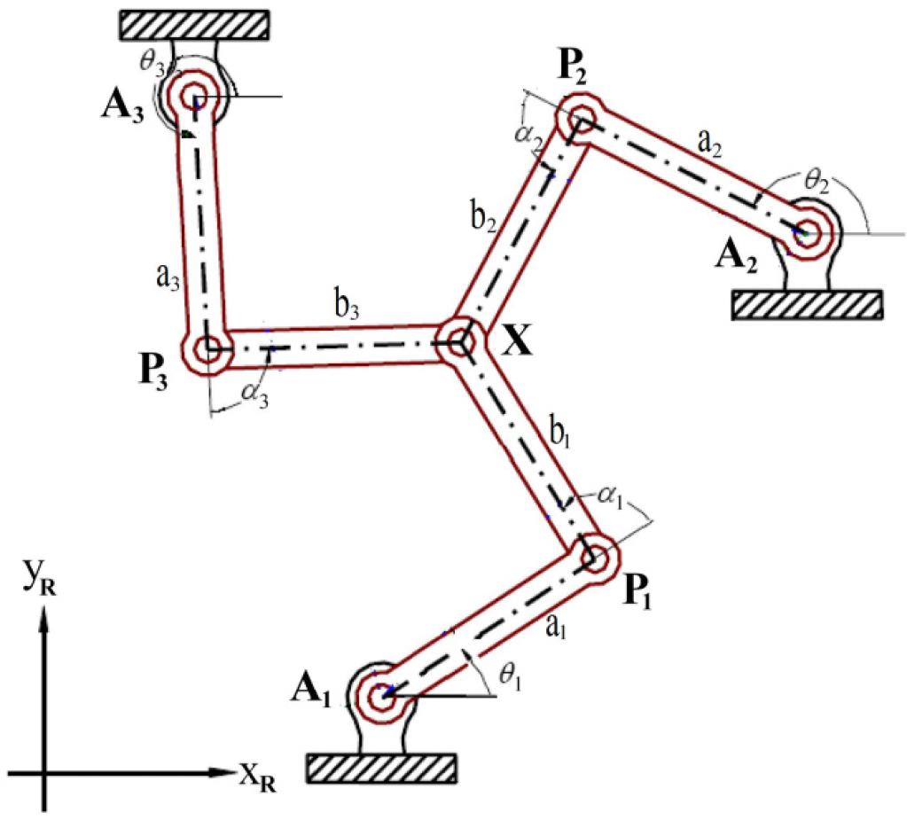
Planar parallel robot.
According to [36], the Lagrange-D'Alembert formulation yields a simple scheme for computing the dynamics of redundant parallel robots; this approach uses an equivalent open-chain mechanism shown in Figure 2. Thus, the dynamics of the parallel robot are equivalent to the dynamics of the open-chain system and a set of loop constraints.

Equivalent open-chain mechanism
The well-known Euler-Lagrange formalism [49] allows the modelling of the open-chain system when the parallel robot moves in the horizontal plane:
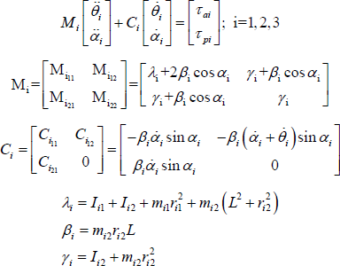
The model above assumes that all the links have the same length – i.e., L = ai= bi. The parameters Iij, mij and rij correspond, respectively, to the inertia, mass and centre of mass of each link. As can be seen in Figure 2, τa = [τa1 τa2 τ a3]
T
stands for the active joint torques and the vector τp = [τp1 τp2 τp3]
T
corresponds to the torques in the passive joints. The neglect of the friction in the passive joints permits the setting
The following is a compact representation of model (1):

The terms
It is worth mentioning that model (2) describes the parallel robot dynamics in terms of the passive and active joint coordinates. However, since the proposed control law uses visual measurements of the robot end-effector position

The terms
The following expressions define the Jacobian matrices


Note that the Jacobian matrix

The vector

Substituting the input torque (2) into (3) leads to:
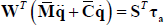
Substituting (6) and (7) into (8) produces the following dynamic model:

The matrices

2.2 Modelling of the vision system
Consider the redundant planar parallel robot described previously. Figure 3 shows the vision system configuration.

Camera and robot workspace
Here, a camera provides an image of the robot workspace, including the robot end-effector. The camera optical centre is located at a distance z with respect to the robot coordinate frame xR – yR and the camera optical axis intersects this frame at the point

Robot and camera coordinate frames
The variable β denotes the camera orientation measured clockwise with respect to the negative side of axis x
Using the perspective camera model [4], [43] allows the description of the end-effector position

The vector

The parameter f is the camera focal length and

The time derivative of (11) gives the end-effector linear velocity in terms of the image coordinate frame as:

The next relationship describes the desired end-effector position

The visual distance between the end-effector image position and the desired end-effector image position (see Figure 5) defines the image position error Image position error

Assuming a constant desired position and taking the time derivative of the image position error yields:

3. Visual Control using only position measurements
3.1 Problem statement
The following statement defines the control problem: given just those measurements provided by a vision system and the robot joints, design a control law generating active joint torques τ
The next expressions permit the computing of the active torques τ

The matrix (

The matrix (
Replacing

Therefore, the control laws discussed below will be defined in terms of the control signal
3.2 Proposed control law
First, consider the following visual servoing PD control law [48]:
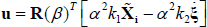
Where k1, k2 and α are positive constants. The fact that the camera orientation β is unknown precludes the use of control law (21) and (22). Assume that only an estimate β of β is known, with –π /2 < β < π /2, this permits the rewriting of (21) and (22) as:
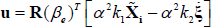

Hence, (18) allows the computation of the control active torque τ
a
as follows:


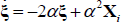
Substituting (23) into (20) leads to the following closed-loop dynamics:

Adding and subtracting the right-hand-side of (21) to the right-hand-side of (27) yields:

The term
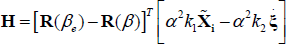
The first term in the right hand side of (28) corresponds to the nominal closed-loop system with known camera rotation. The vector

3.3 Stability analysis
Defining the state vector

An equilibrium point for the closed-loop system (31) is
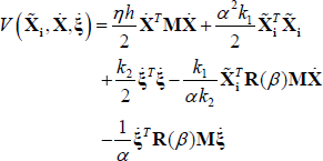

The above function is a radially unbounded positive definite, provided that the following terms:


Let us consider the following bounds:

Hence, the terms (33) and (34) satisfy:
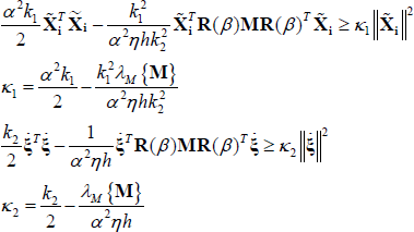
From the above, it is clear that for a value of α which is large enough, the terms (33) and (34) are positive definite functions.
Therefore, the Lyapunov function candidate (32) is radially unbounded and positive definite.
The following expression corresponds to the time derivative of (32) along the trajectories of the closed-loop system (31):
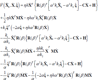
Using
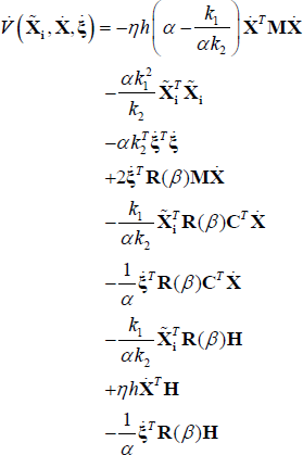

The above bounds permit, in turn, the bounding of the time derivative (35) as follows:

In order to obtain a compact writing of (36), let us define the vector

The matrix

At this point of the analysis, it is convenient to establish the next inequalities obtained from (32) and the definition of vector ψ:
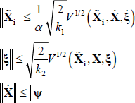
Hence, it is not difficult to show – using the above inequalities – that the term Γ has the following upper bound:

Finally, using the above bound leads to the following inequality:

The term V(t) in (39) is a simplified writing of
When ρ = 0 for a given initial state

Then, there exists a non-zero value ρ* small enough fulfilling:

With b(α*, 0,0) >b(α*, ρ*, 0). Note also that the relationship

Therefore, choosing the initial conditions for the Lyapunov function

Consequently, applying the second Lyapunov stability method [50] permits the conclusion that the equilibrium point
4. Experimental Results
The 3-RRR redundant parallel manipulator shown in Figure 6 serves as a test bench for evaluating the proposed visual controller. The link lengths of this prototype are L=15cm. Brushed servomotors from a Litton PolyScientific – model C34L80W40 – drive the active joints through timing belts with a 3.6:1 ratio. Pulse width modulation digital amplifiers from Copley Controls – model Junus 90 working in current mode – drive the motors. Absolute magnetic encoders from US Digital – model MA3 – with a resolution of 10 bits, supply the measurements of the robot active and passive joint angles θi and α
i
that are used for computing (
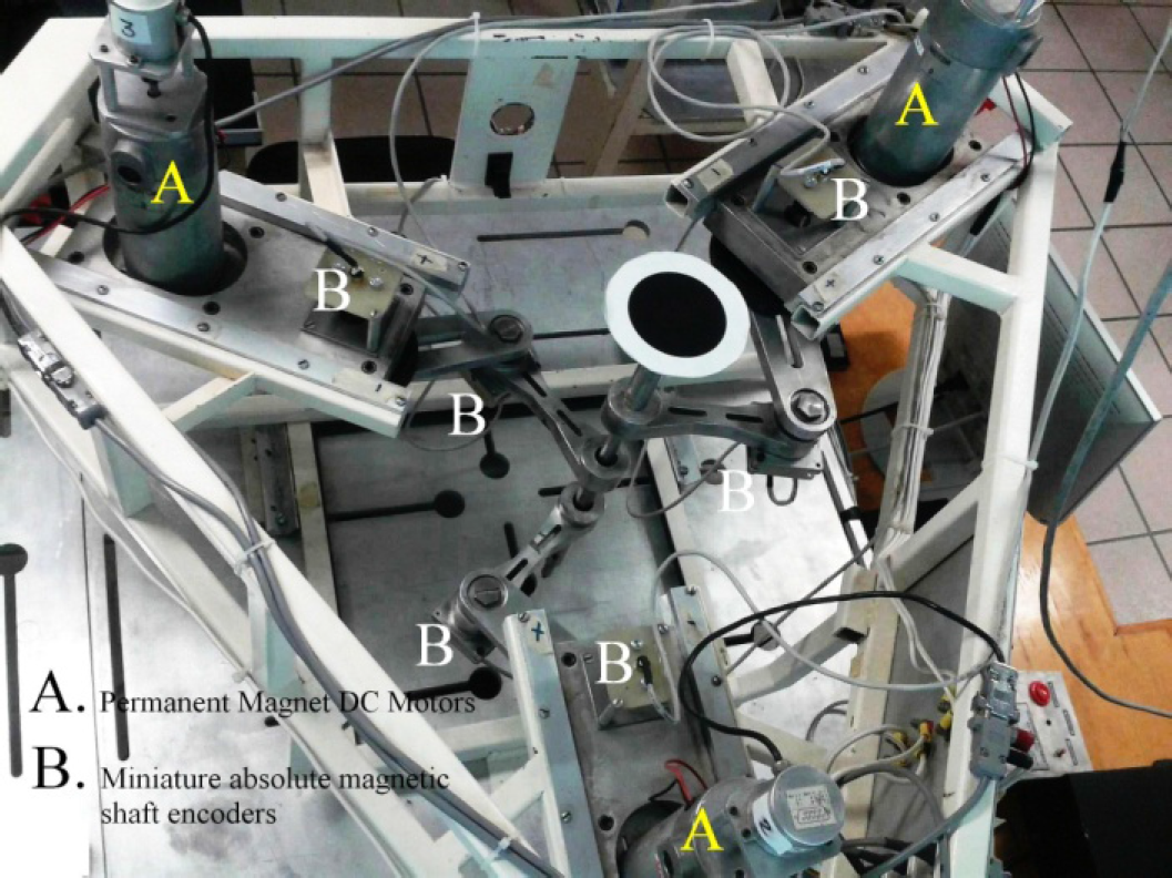
Laboratory prototype used in the experiments
In order to evaluate the performance of the proposed control laws (25) and (26) under uncertainty in relation to camera orientation, this section presents two sets of experiments. The first set considers β = 0 rad and βe = 0 rad – i.e., the robot and camera coordinate frames are parallel (see Figure 7). In the second set of experiments, the real and estimated camera orientation are different; their respective values are β = π/6 rad and βe = 0 rad (see Figure 8). The controller gains used for both sets of experiments are k1 = 7.26 × 10³, k2 = 1.46×10⁻⁴ and α = 150. The reference

Image of the robot workspace without camera rotation

Image of the robot workspace with camera rotation
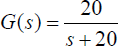
with a frequency of 0.1 Hz plus a constant signal of 80 pixels. Reference y*i is also a square wave of 16 pixels of amplitude with a frequency of 0.1 Hz plus a constant signal of 75 pixels. The following linear filter:
In the case of the first set of experiments, Figure 9 shows the time evolution of the end-effector coordinates and Figure 10 depicts the corresponding image position errors; Figure 11 portrays the active joint torque signals.

Closed-loop system response for β = 0

Image position errors for β = 0

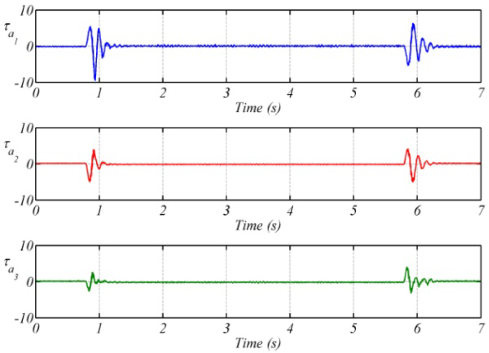
Active joint torques for β = 0
The above results show that the closed-loop response has almost no oscillations; the position errors remain around 1 pixel and the active torque signals do not exhibit a high level of high-frequency components.
For the second set of experiments, the time evolution of the end-effector coordinates depicted in Figure 12 has essentially the same behaviour as that observed in the first set of experiments; a similar observation may be made for the position errors shown in Figure 13 and the active joint torques portrayed in Figure 14. It is clear from the results of both sets of experiments that the uncertainty in the camera orientation does not have a significant impact on the closed-loop response, with only a slight increment in the position error.

Closed-loop system response for β = π/6

Image position errors for β = π/6
Active joint torques for β = π/6
5. Conclusions
The theoretical and experimental results discussed in previous sections show that the visual control algorithm studied here – which essentially behaves like a classic PD algorithm – is able to withstand uncertainties in camera orientation. This algorithm does not rely on velocity measurements and has low computational requirements. On the theoretical side, a key element in the stability analysis is a strict Lyapunov function that includes the camera rotation matrix; this function allows the establishment of asymptotic stability without relying on the invariance set stability theorems. On the experimental side, the results obtained using a laboratory prototype show that the closed-loop performance remains essentially the same when the camera rotation is unknown for the controller.
Footnotes
6. Acknowledgments
The authors would like to thank Gerard Castro and Jesús Meza for setting up the laboratory prototype