
Abstract
This paper elaborates upon a musculoskeletal-inspired robot manipulator using a prototype of the spiral motor developed in our laboratory. The spiral motors represent the antagonistic muscles due to the high forward/backward drivability without any gears or mechanisms. Modelling of the biarticular structure with spiral motor dynamics was presented and simulations were carried out to compare two control methods, Inverse Kinematics (IK) and direct-Cartesian control, between monoarticular only structures and biarticular structures using the spiral motor. The results show the feasibility of the control, especially in maintaining air gaps within the spiral motor.
Keywords
1. Introduction
Over recent decades robots have been inspired by the motion of living things, i.e., humans and animals [1] [2]. Various structures of robots have been designed, from industrial robotic manipulators to humanoids and mobile legged robots for different purposes. Success stories include ASIMO, DLR, Big Dog and many others. However, most designs are implemented by using serial joint servos at the end of each limb, resulting in large joint actuators at the base to support the desired large forces/torques (i.e., end-effector output, friction). In the end, the weight and size of the actuators contribute largely to the overall specification of the robot. In addition, difficulties in actuation, for example, backlash and low drivability/low compliance, add to problems in controlling such structures.
On the other hand, the anatomy of the musculoskeletal human body provides new insights into the design of robots. By looking closely at the structure of the human/animal musculoskeleton, the joint/hinges are not directly actuated, but affected by the antagonistic contraction or extension of the muscles connected to the bones. The muscles can be clustered into monoarticulars (single joint articulated) and biarticulars (two joint actuated). The dynamic domain of the human arm muscles (from shoulder to elbow) have been studied in [3] [4] [5]. The study in [3] applies the Hill's muscle model and attempted to analyse different damping and elastic properties, and later applied task position feedback control to monitor position, velocity and accelerations in joint and taskspace. On the variation of muscle positioning, the potential fields produced by the internal forces are affected and also the speed of convergence of motion. By means of simulation, the human reaching movements were achieved without inverse dynamics or optimal trajectory derivation.
Some designs that include biarticular muscle actuation can be referred to in [6] and [7]. These designs use rotary motors, belts and pulleys to realize biarticular muscle torques. In [6], stiffness and inverse dynamics feedforward control was applied. The lancelet (ancestor of the vertebrae) has inspired [7] using similar mechanisms to realize a virtual triarticular sigmoid/swimming motion with the properties of AC motor control. These designs include the biarticular/triarticular actuation, but the structures are maintained as serial or open-link mechanisms. Another different design was shown in [8], whereby the rotary motors are placed at the base and the joint angles are pulled by wires. Feedforward control was also applied to resolve force redundancy. Other designs of legged musculoskeletal mechanisms can be found in [9] [10] [11]. These structures utilize the pneumatic rubber muscles as actuators, possibly the closest candidate to the human muscle. These muscles extend or contract, depending on the amount of air pressure supplied. The small size of the actuators enables the design of the legs to be space saving, as the actuators are placed closely or attached to the link. Jumping and hopping motions were successfully implemented, but because of the use of air supply, these structures are less mobile for autonomous operations. Also, pneumatic muscles are difficult to control and inaccurate due to their nonlinear elasticity properties [12]. A combination of pneumatics/cables is also shown in [13].
The actuator that we propose for musculoskeletal actuation is the spiral motor [14]. It is a novel high thrust force actuator with high forward/backdrivability. From the first prototype, the internal permanent version was developed and currently the helical surface permanent magnet prototype is available [15].
2. Biarticular Manipulator Kinematics
An example of the biarticular muscle structure can be found in the human arm, consisting of antagonistic pairs of monoarticular (muscles affecting one joint) and biarticular muscles (muscles affecting two joints). By using the spiral motor, the antagonistic pair of flexor and extensor can be combined by using only one spiral motor, thus reducing the number of actuators from the shoulder to the elbow to only three actuators, instead of six. The combined flexor/extensor muscles of the planar manipulator of the biarticular structure is shown in Figure 1.

Simplified diagram and manipulator design
The main angles are the shoulder angle (q1) and elbow angle (q2). Based on the simplified diagram in Figure 1 and using trigonometric identities, the relationship of muscle lengths, lmi with joint angles q1 and q2 is derived (a 1 and a2 are link lengths).

Distances between connection lengths of the monoarticulars from the joint angles are labelled al1, al2, bl1 and bl2 while connection lengths of biarticular are al31 and al32. The extension/contraction of monoarticular muscles affect the respective joint angles to which they attach, i.e., lm1 affects the joint angle q1 (shoulder) and lm1 affects q2 (elbow). However, the biarticular muscle lm3 is redundant because it affects both q1 and q2.
Based on (1), the relation between muscle velocities,

Where Jlmq is the muscle-to-joint space Jacobian, obtained from partial derivatives of (1) with respect to shoulder and elbow angles, shown in (3).

where

It needs to be highlighted that this Jacobian is different from that of [6], because in the mentioned reference it is not structure-dependent. In our case, this Jacobian varies with the connection points (i.e., al1, al2, bl1, bl2, al31 and al32). Next, the equation relating joint torques, τ (vector of shoulder and elbow torques) and muscle forces,

Also, the equation relating the joint torques, τ and the end-effector forces,
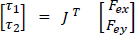
where J is the 2R planar Jacobian matrix from task space to joint space which contains the following elements;

The equation relating to the end-effector forces,

From Equation (6), the end-effector forces plot of the biarticular structure can be obtained. Figure 2 shows the static end-effector forces of structures with biarticular forces and the structures without. The forces applied for lm1 [N], lm2 [N] and lm3 [N] are;
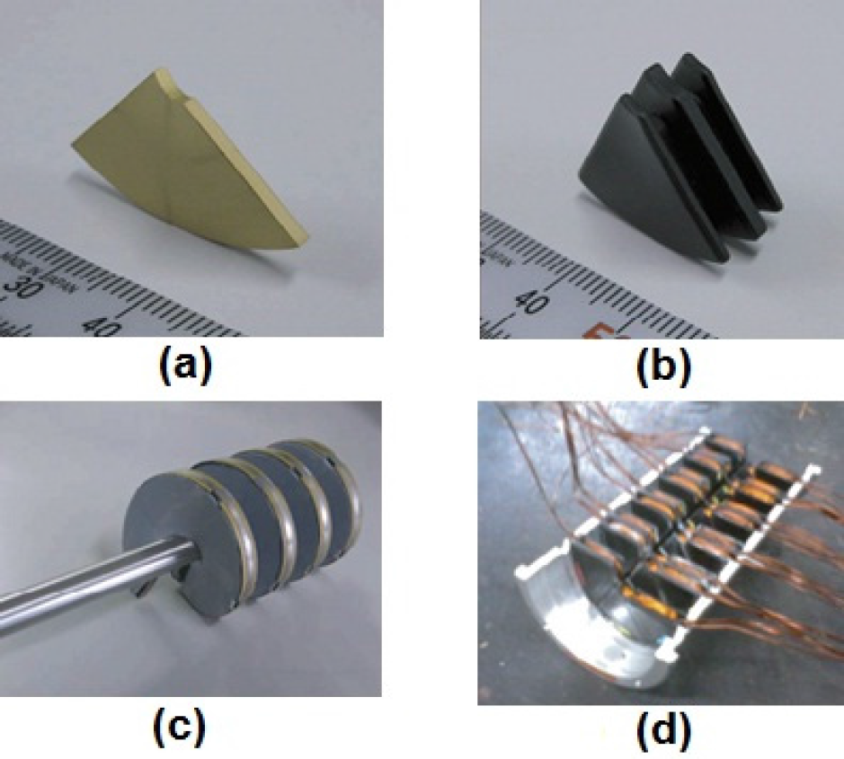
Cartesian view of end-effector forces for structures with (red) and without (blue) biarticular muscle forces Spiral motor parts (a) Neodymium magnet (b) Silicon steel stator yoke (c) Mover attached with magnet and Teflon sheet (d) Wound and assembled half stator

The end-effector output force produced by biarticular forces shows a hexagonal shape which is more homogenous than the tetragonal shape of the end-effector forces without biarticular actuation. This is one of the many advantages of biarticular manipulators compared to monoarticular actuation only.
3. The Spiral Motor
Being specifically developed for musculoskeletal robotics, the third prototype spiral motor's main feature is its direct drive high thrust force actuator with high backdrivability. This three phase permanent magnet motor consists of a helical structure mover with permanent magnet and stator. The linear motion is derived from the spiral motion of the mover to drive the load. In addition, the motor has high thrust force characteristics because the flux is effectively utilized in its three dimensional structure [14]. This spiral motor does not include ball screw mechanisms, thus friction is negligible under proper air gap (magnetic levitation) control.
As seen in Figure 4, there is a small air gap between the mover and stator. This small distance is ideally 700 um between the Teflon sheet of the mover (at centre position) and the stator yoke. This air gap displacement, xg, is related to the linear displacement, x, and angular displacement, θ, in (11). If the gap displacement is maintained, i.e., the surface of mover and stator are untouched, magnetic levitation is realized. Simultaneously, by a vector control strategy, the angular control provided by q-axis currents will give forward or backward thrust while d-axis currents control linear displacements and magnetic levitation, as shown in the plant dynamics of the spiral motor in (9) to (12);
Spiral motor illustration Assembled short-length spiral motor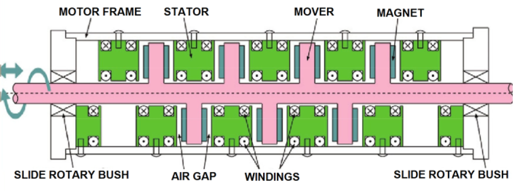


where
3.1 Direct Drive Control of the Spiral Motor
Assume uxg and uθ are control inputs for gap displacement and angular displacement [15], which will match its respective acceleration terms;


where xq0 is the gap reference and ẋq0 is the gap velocity reference. Kpg, Kdg, Kpt and Kdt are PD gains for gap and angular positions and velocities. Also, the relation between linear and angular acceleration is known as;

By replacing the linear acceleration term in (9) with (15), force dynamics of (9) can also be expressed as;

Replacing the acceleration terms with control inputs (subscript n denotes nominal value);

Thus, the d-axis current reference (that will be tracked by a PI current controller) will have the following form;
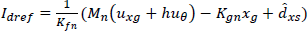
By applying the same technique to the torque dynamics in (9) for the q-axis current reference;


where gx and gθ are the gain of the disturbance observer for linear and angular displacements. Until this point, direct drive control can be achieved at gap values of 0 mm. But due to disturbances (i.e., manufacturing accuracy of mover and stator), the current at 0 mm is not zero. Therefore, a neutral point (zero power) that induces zero currents for d-axis current is desired and low power control is realized as follows;

As acceleration terms are usually affected by noise (due to differentiation), for initial testing, we simplify (24) to become;

Experiments for direct drive forward and reverse motion were carried out using the monoarticular spiral motor with a stroke of 0.06 m. TMS320C6713–225MHz were used for data collection and control. Two DC supplies for the forward and backward inverters were used. At first, the direct drive control was applied to 0 mm (x position). We regard this as the initial gap stabilization phase. This is required because once magnetic levitation is realized, then forward and backward motions can be performed smoothly. If magnetic levitation and forward/back motions are performed simultaneously, the gap might not be maintained and damage could be inflicted on the stator and mover. After d-axis current stabilized at around 0 A, the forward reference was given. Then after the current stabilize at 0 A again, the reverse reference of 0 mm was applied. Figure 6 shows the experimental results for direct drive forward/reverse motion with zero d-axis current control (after gap initialization). Note that in [15], direct drive control was performed without zero d-axis control.

Direct drive experimental results with zero d-axis current control (a) Forward drive (b) Gap displacements (red denotes zero d-axis gap reference) (c) Currents (d) Reverse drive (e) Gap displacement (f) Currents
4. Singularity/manipulability of Biarticular Structure
This kinematic parameters can be used to determine the work space of the manipulator. The parameters of the three spiral motors are shown in Table 1.
Spiral motor specifications for muscles

The forward kinematics (end-effector position) of a 2R manipulator can be calculated by using the following equation (x and y are Cartesian coordinates);


For the biarticular manipulator, kinematic limits are due to the maximum (α2, β2) and minimum length (α1, β1) of the actuators, shown as;

By referring to Equation (1), joint angle q1 is bounded to the connection lengths al1 and al2. The same applies for monoarticular lm2. For us, we chose al1 = bl1 and al2 = bl2 (same arrangement for both monoarticulars).
Then, the ranges of allowable angles for q1 and q2 are;
where

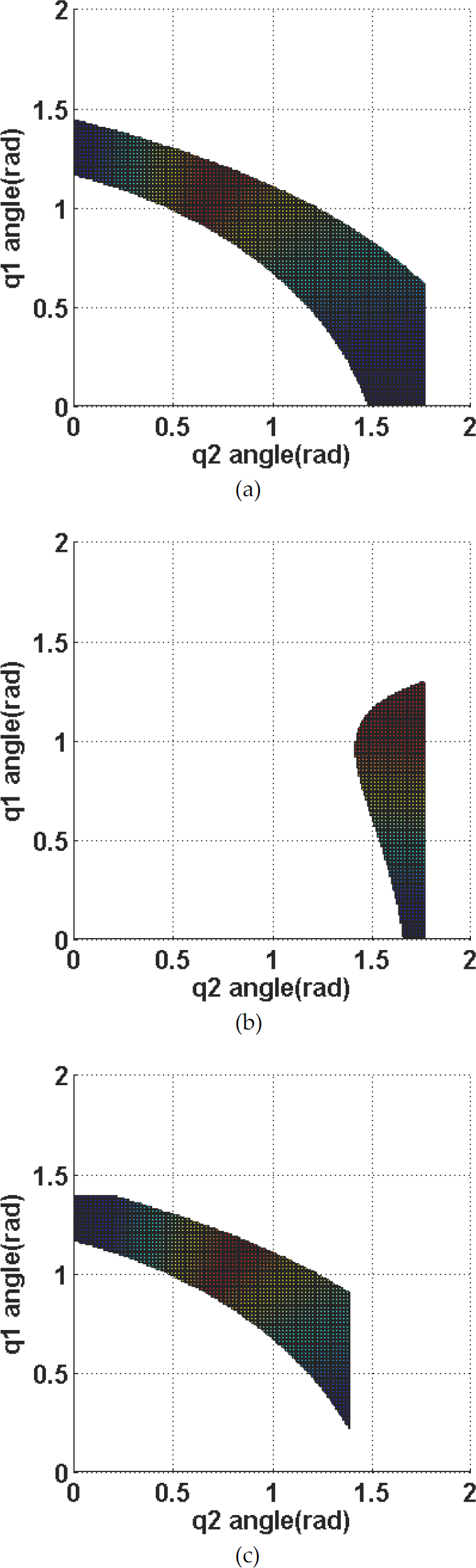
This implies that the minimum lengths of monoarticulars incur maximum angles and vice versa. Thus, considering biarticular length limits, manipulability [16] can be plotted. Figure 8 shows the manipulability plots for different connecting points of monoarticular muscles. The shape of the angle limits is due to biarticular and monoarticular length limits. It can be seen that the further the connection points of monoarticulars are from the shoulder angle, the larger the work space.
Manipulability was obtained by finding the determinants of the muscle-joint Jacobian and end-effector-joint Jacobian terms. Dark blue represents low manipulability regions, and at zero manipulability, singularity is induced. Red represents the high manipulability region.
The inverse kinematic singularity of planar 2R manipulator [24] can be seen at the elbow angle of 0 radians. This is also true for the biarticular manipulator. In addition, due to muscle Jacobian terms, singularity is also evident at the shoulder angle of 0 radians. Some examples of singularity and manipulability poses for the biarticular manipulator are illustrated in Figure 9.
In the case that either shoulder or elbow monoarticular becomes fully extended, the shoulder/elbow angle becomes zero, and singularity is observed. However, both angles could not become zero simultaneously, due to biarticular length limit (refer Figure 7).

Closed-kinematics of biarticular manipulator

Manipulability plots for (a) al1=0.14m, (b) al1=0.16m, (c) al1=0.18m and (d) al1=0.20m for similar elbow monoarticular connection (al1 = bl1). Biarticular connections (al31 and al32) set at 0.06 m

Examples of singular and manipulability poses for biarticular structure.
Higher manipulability poses are induced when lengths of muscles are short, and at near minimum lengths of muscles (or maximum angles), maximum manipulability region is observed.
If the connection points of shoulder and elbow monoarticulars are different, the following results of reciprocal condition of the Jacobian (another method to determine ill-condition [25]) is shown in Figure 10 and Figure 11;

Reciprocal condition plot for al1 ≠ bl1, al1 = 0.2 m bl1 = 0.14 m; (a) al31 = al32 = 0.06 m (b) al31 = al32 = 0.10 m

Reciprocal condition plot; al1 ≠ bl1, al1 = 0.14 m and bl1 = 0.2 m; (a) al31 = al32 = 0.06 m (b) al31 = al32 = 0.10 m
As seen in Figure 10 and 11, if the value of al1 or bl1 is small, the corresponding shoulder/elbow angle becomes narrow and vice versa. Also, the further the biarticular muscle connection point is from the hinges, the smaller the work space becomes. By increasing the biarticular connection distance, ill-condition is further avoided, but with less work space.
Figure 12 shows the reciprocal condition plot with different connection points of the biarticular muscle. It is obvious that by connecting the end of each side of the biarticular muscle differently, significant changes to the work space and reciprocal condition is seen.
Reciprocal condition plot; al1 = bl1 = 0.2 m; (a) al31 = 0.06 m, al32 = 0.10 m (b) al31 = 0.08 m, al32 = 0.06 m; (c) al1 = bl1 = 0.14 m al31 = 0.06 m, al32 = 0.10 m
5. Biarticular Plant Dynamics Modelling
Most planar 2R robots are serial/open-chain manipulators. There is much research on control of these 2R manipulators. Modelling of unconstrained open-chain manipulators uses Ordinary Differential Equations (via Lagrange (LE) or Newton Euler (NE) formulation), while closed-chain manipulators require Differential Algebraic Equations due to constraint equations [17]. Constraint points are virtually cut open and LE formulation was used to obtain mass, gravity and centrifugal matrices. Equation (29) depicts the generalized equations of motion of a closed-chain manipulator;

where
Constraint equations (from trigonometry) are derived as;

Also, the relative acceleration at the constraints are zero (Jc, J̇c are the constraint Jacobian and Jacobian derivative),

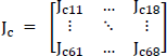
The constraint Jacobian (unmentioned terms are zero) is described as;

The constraint Jacobian derivative is derived as;


By combining these two equations, the following generalized closed-chain model can be derived;

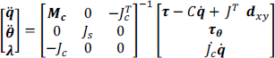
To include the spiral motor plant dynamics in the generalized closed-chain model, (33) has to be modified to the following;

The inertia terms from the angular rotation now emerge (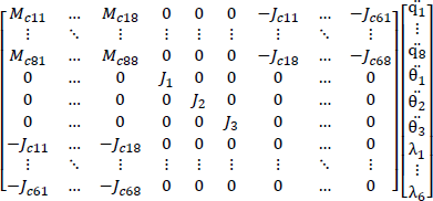
The linear acceleration of the spiral motors (i.e.,
The right-hand terms of (34) would become;
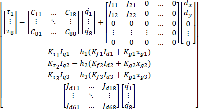
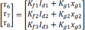
The unactuated variables are q1 to q5. Thus, its corresponding τ1 to τ5 are always 0 (no input torque/force). τθ is the vector of spiral motor torques. τ6 to τ8 (monoarticular 1, monoarticular 2 and biarticular forces) are given by the following equation;
In simplified terms, the plant can be described by (38);
6. Work Space Position Control
Robotic manipulators have been researched extensively; some of the many examples are torque sensorless control [18], SCARA manipulator tracking control [19], feedforward and computed torque control [20] and position control of constrained robotic system [21]. Previously described in [22] are some approaches (the IK approach and the Direct Cartesian (DC) approach) for the general structure of a biarticular manipulator, i.e., not actuator specific. In [23] other methods were investigated.
In this paper, the generalized work space control [22] is extended to the specific spiral motor case for the purpose of viewing the effects on gap and position control with the addition of Cartesian load disturbance. By considering a circular task space trajectory, the references for x and y-axis positions are shown as;

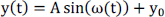
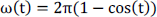
where A is the radius of the circle and x0 and y0 are x and y coordinates of the centre of the circle.
From 0 to 0.5 seconds, gap stabilization is performed without giving any position reference (either in joint space or work space). This phase is to allow the gap to stabilize at centre (0mm) position. From 0.5 to 6 seconds, the position reference of the circle trajectory (5 cm radius) is given. In addition, Cartesian disturbance on the end-effector is given between 1 to 3 seconds.
Here we present comparisons of a monoarticular only actuated structure with that of a biarticular structure by using the IK approach and the DC approach (monoarticular control gains, i.e., PD, disturbance observer cut-off frequencies are identical). Note that for work space control, zero d-axis current control is not applied.
5.1 Inverse Kinematics Approach
By using the IK approach [24], joint space trajectories (elbow/shoulder angles) are obtained from the Cartesian reference trajectories (x and y);


From joint references, muscle kinematics (1) can be used to obtain muscle references (i.e., length, velocity, acceleration). ẍ1, ẍ2, ẍ3 are shoulder, elbow monoarticular and biarticular spiral motor linear accelerations.


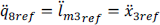
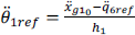
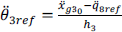
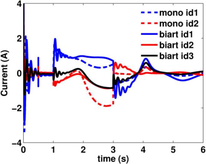
The rotational acceleration references are calculated as in (48) to (50) with
From these references, dq-axis control (refer (13) to (20)) can be constructed for each muscle to generate the forces (τ6, τ7, τ8) and torques (τθ1, τθ2, τθ3) as in (36) and (37).
In this part, only Y-axis disturbance of 10 [N] is given. The initial circle trajectory response in Figure 14 shows that the biarticular structure exhibits better accuracy. Initial errors due to the gap stabilization can be seen at the near start position (0.15, 0.53). Then the effect disturbance of 10 [N] can be seen as the response is deviating from the reference. Cartesian errors are shown in Figure 15; ‘mono’ denotes monoarticular structure responses while ‘biart’ denotes biarticular structure responses.

IK control for manipulator driven by spiral motors

Close-up view of circle trajectory responses from monoarticular structure and biarticular structure

Cartesian errors for the IK approach
For Figure 16, ‘mono gap1’ and ‘mono gap2’ refer to the monoarticular muscle gaps in the monoarticular structure, while ‘biart gap1’, ‘biart gap2’, ‘biart gap3’ refer to the shoulder monoarticular gap, elbow monoarticular gap and biarticular gap in the biarticular structure. Referring to gap displacement responses in Figure 16, in the initial gap stabilization phase (0 to 0.5 s), more interaction is obvious in the biarticular case, but the biarticular structure shows better gap control during position tracking.

Gap responses for the IK approach
Force responses from muscles are shown in Figure 17. Both forces are bounded. Next, the torque responses (rotational part of spiral motor) are shown in Figure 18.

Spiral motor forces for the IK approach

Spiral motor torque for the IK approach
Figures 19 and 20 show the d- and q-axis currents generated. As in the spiral motor simplified plant model, the d-axis is related to muscle (spiral motor) forces while the q-axis is related to spiral motor torques. It can be said that the biarticular forces reduce the effort of the elbow monoarticular muscle, but increase shoulder muscle actuation.
D-axis current for the IK approach

Q-axis current for the IK approach
For this approach, muscle force interactions are clearly visible (seen in oscillations) as expected, because the muscles are independently controlled without any force distribution.
5.2 Direct Cartesian Approach
For the DC approach, the forces from work space/task space domain are controlled in the shoulder and elbow joint space (virtually), then transferred to the actuator (muscle) space by the joint-muscle Jacobian (3).
Figure 21 shows the control diagram and the control equation is shown in Equation (51) to (55). xres, yres are Cartesian end-effector position responses.

DC control for manipulator
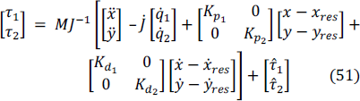


where

The inverse Jacobian to obtain the muscle forces, Flml are calculated by using Moore's inverse pseudomatrix. ẍ is Cartesian acceleration, J−1 is the inverse of (6), J̇ is the Jacobian time derivative, M is 2R planar mass matrix and gi are disturbance observer gains. Now that the muscle forces' terms are obtained from the virtual joint torques, it must be distributed to the gap and angular terms of the spiral motor. From Equation (16), the linear forces for the spiral motor is again shown;

The gap control variable (uxg) is the same as in (13), but the angular control variable is obtained by manipulating Equation (54) (subscript i refers to respective muscle number);

For this study, Cartesian Y disturbance of 10 [N] is also added to the end-effector from the period of 1 to 3 seconds. The trajectory tracking and Cartesian errors are depicted in Figure 22 and Figure 23 which shows significant improvements compared to the IK approach.
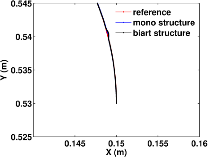
Close-up view of circle trajectory responses for the DC approach

Cartesian errors for the DC approach
Next, the gap responses are shown in Figure 24. Biarticular muscle helps reduce gap values for monoarticulars, especially during disturbance.

Gap responses for the DC approach
The spiral motor force and torques are depicted in Figure 25 and Figure 26. Forces were acceptable and bounded between 60 [N] in both directions for all the muscles.

Spiral motor forces for the DC approach

Muscle torques for the DC approach
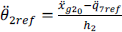
Next, spiral motor d- and q-axis currents are shown in Figure 27 and Figure 28. It can be seen that the d-axis current is lower in the biarticular structure than in the monoarticular only structure.

D-axis current for the DC approach

D-axis currents for the DC approach
7. Discussion
The two methods for position control in the task space/work space domain provide some interesting results. It is clear that the IK approach and the DC approach yield acceptable responses.
In the gap stabilization phase, IK provides a clear oscillatory response in achieving a gap at the centre (0 mm). The biarticular actuation increases the oscillations of the gaps. In the DC approach, this oscillation does not exist, in both monoarticular and biarticular structures. The DC approach provides smooth gap responses initially. At the start of position tracking (before disturbance), both methods yield good responses (i.e., variation of gap minimum, small amount of forces and currents), but during disturbance, the effects can be seen clearly. Tracking errors increase, but control was maintained. Towards the end of the disturbance, errors were acceptable.
Table 2 summarizes the comparisons of the IK and DC methods on monoarticular and biarticular structures based on Cartesian errors.
Comparison of errors between methods/structure

In short, errors for DC method are lower than IK method and errors for biarticular structures are lower than monoarticular structures.
8. Conclusion and Future Works
This paper has shown the proposed biarticular manipulator using spiral motors developed in our laboratory. The simplification and arrangements of the muscles and the end-effector-muscle-joint force properties were initially presented. Then, the spiral motor was introduced and manipulability was discussed. Next, the modelling of the biarticular manipulator using spiral motors was briefly explained and the results of the IK approach and the DC approach for position control of the manipulator were compared between a monoarticular only structure and a biarticular structure. For work space force control schemes (with environment) of a biarticular manipulator, readers are advised to refer to [26].
The gap control is a crucial element in the spiral motor direct drive motion. It was shown that the work space position control was successful in all cases, although some better responses were shown in the biarticular manipulator. Among the advantages of the biarticular structure were the improved control of the gap of the elbow monoarticular muscle and better accuracy of trajectory tracking. In future, we plan to compare our manipulator to other biarticular manipulators available, i.e., ball-screw mechanism, pneumatics, cables or hydraulics.
Footnotes
9. Acknowledgments
This work was supported by KAKENHI 24246047.